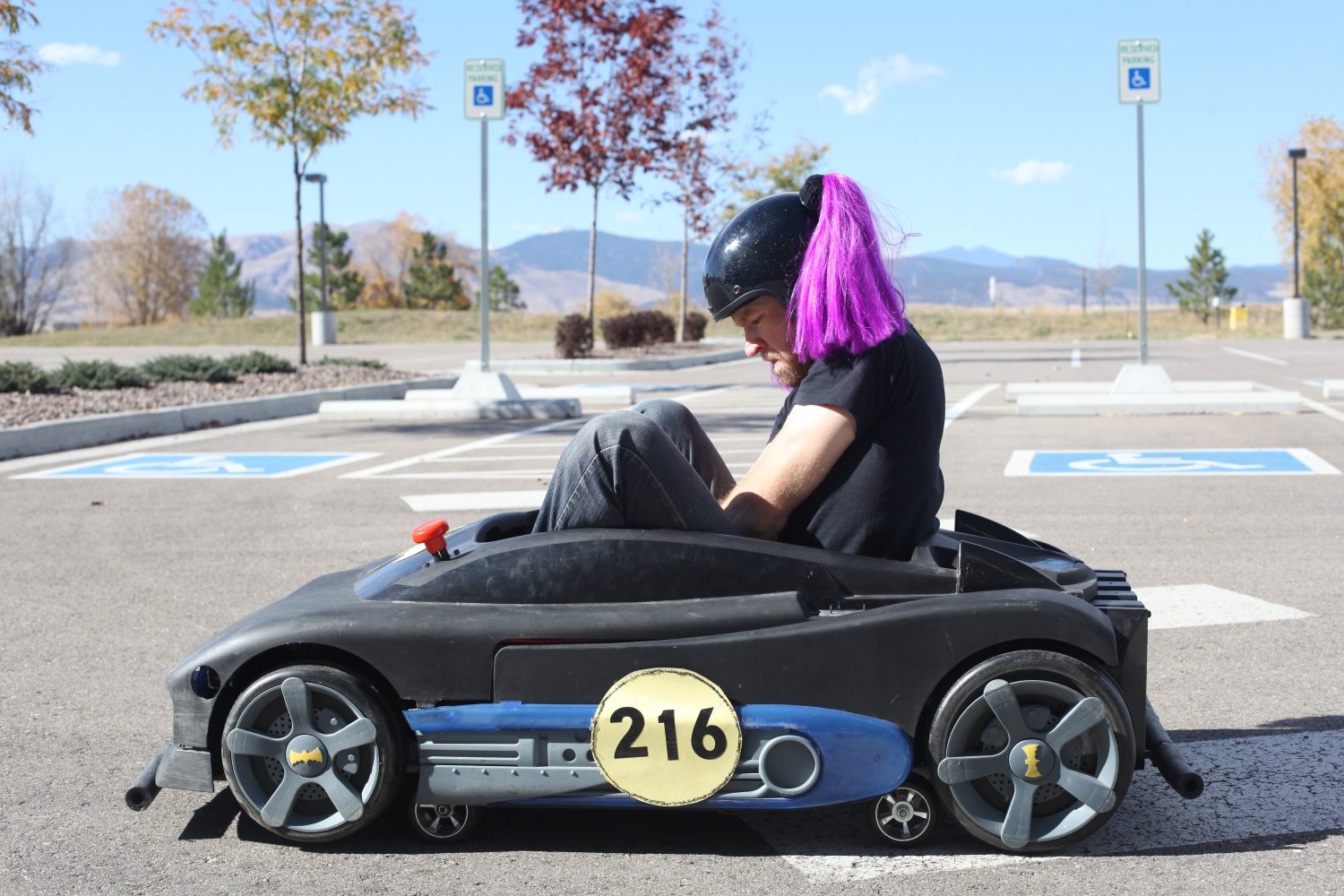
Bygga en egen autonom bil – The Batmobile

Test driving the Batmobile

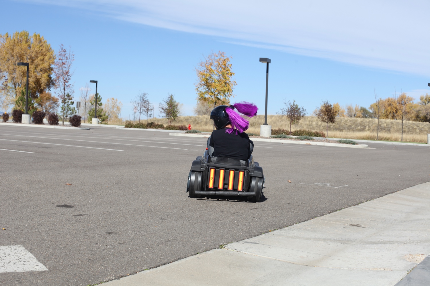
The thrill of taking a corner, extremely low to the ground, with your gut telling you these g-forces are not normal… that’s why we spend countless hours building these silly Power Wheels vehicles. The giggles and grins are unavoidable! These cars are so much fun to drive — and even more fun to race!

In 2016, SparkFun had its eighth annual Autonomous Vehicle Competition. This year saw the introduction of a new rule: you needed to carry a human (or a 20lb dead weight in the form of a watermelon if you were too chicken). To do this, my wife, Alicia, and I modified a Batmobile Power Wheels and combined it with a Razor chassis. The result was an extremely zippy electric go-kart that left a perma-grin on everyone who drove it.

Our goal was to create a vehicle that could quickly and easily switch between human driver and driverless modes so that we could compete in both PRS and A+PRS categories. In the end, Alicia placed a very respectable third place in the driver category, and I did not finish (DNF) in the autonomous category, running into numerous hay bales.

This tutorial attempts to document a six-month build process for an Autonomous + Power Racing Series (A+PRS) vehicle. Every autonomous vehicle is unique, and the requirements of each will vary from build to build.

Materials

You can see our overall budget, including a list of components and vendors here.A+PRS BATMOBILE MATERIAL SPREADSHEET
You can get all the code from our repo here.A+PRS BATMOBILE GITHUB REPOSITORY

Chassis

The AVC rules stipulate that you cannot spend more than $500 on your total budget and that you have to stay within certain size restrictions. We started trolling craigslist to see what was out there and immediately found a plethora of free or cheap “broken” Power Wheels. When a Batmobile for $25 popped up, we quickly snagged it.

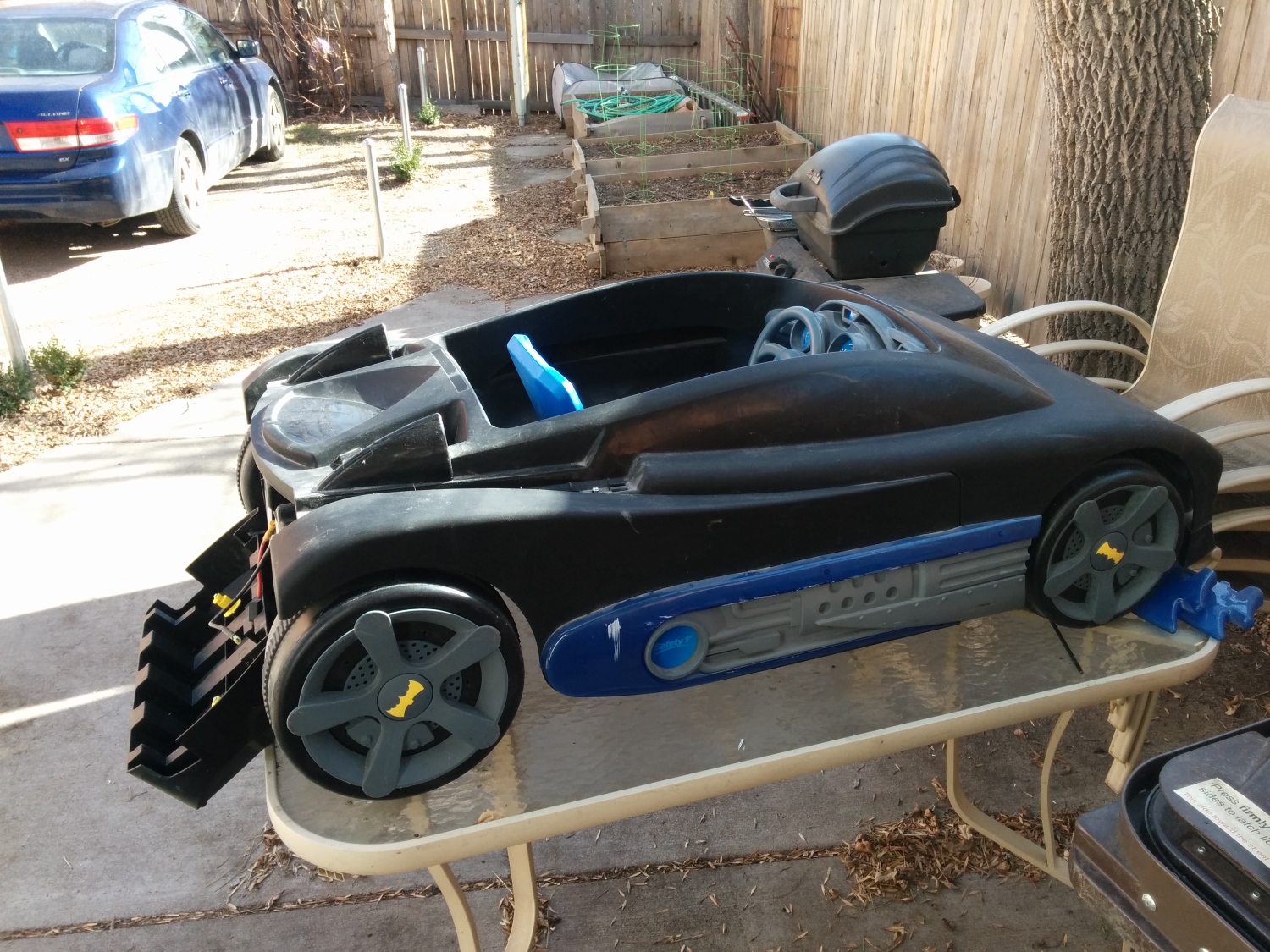
Dusty with dog hair and dead spiders — it’s perfect!

The primary failure of all used Power Wheels is a dead battery. The Batmobile was no different; as soon as we put in a new 12V SLA (Sealed Lead Acid), it happily, albeit slowly, drove around. There is nothing magical about “Power Wheels” branded batteries; get the right voltage (usually 12V, sometimes 6V), and you can use almost any battery you’d like.

The original batmobile chassis blow molded plastic at its finest. The wheels are hollow, the motor is designed to move a child slowly (and reasonably safely), and the steering is littered with bits of metal but mostly loose and wobbly. While the stock chassis was capable of moving adults weighing in at around 200lbs, we knew it wouldn’t handle racing, so we decided to find a metal chassis to sit underneath.

Note the size of the motor and battery. Those are about to get much larger.

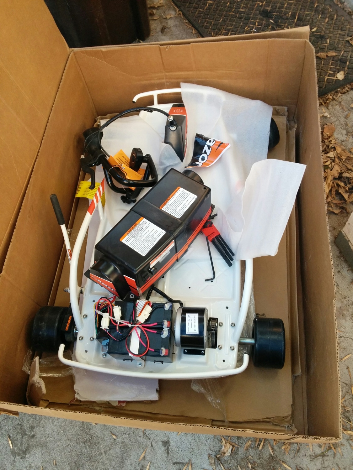
Razor is known for their kick scooters, but they’re in the electric go-kart market as well. We found a Razor Drifter Open Box for $165. The Drifter had the steering, brakes, wheels and chassis sorted out for us! Additionally, the Drifter came with a stock 24V battery, 250W motor and 250W motor controller.

Many PRS and AVC competitors are talented enough to weld their own chassis together. DIY welding is a great way to save money, but it may take weeks of fabrication. Because we planned to enter the autonomous field, we decided to find a ready-made chassis and spend our time building and debugging the autonomous bits.

Putting on a Hat

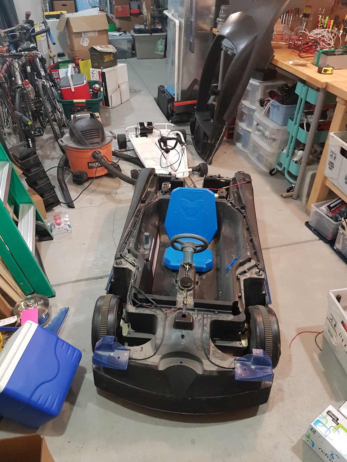
Once we had the Power Wheels and the Razor chassis, we had to combine the two.

We slid the razor chassis underneath the plastic batmobile shell. The razor chassis has strength where we needed it most: steering, chassis, brakes, drive train, everything. The plastic batmobile is just there as a shell. The four solid plastic+rubber razor wheels make contact with the ground. The four hollow batmobile wheels hover above the ground and are there only for cosmetic looks (for the lulz).

A Power Wheels meets a Drifter

At some point you have to get out the reciprocating saw and severely modify your beautiful Power Wheels. We laid the Batmobile over the Razor and proceeded to chop off all the bits that got in the way.

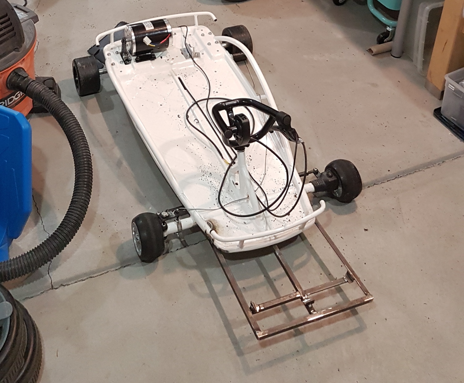
Bare metal chassis before shell is laid on top

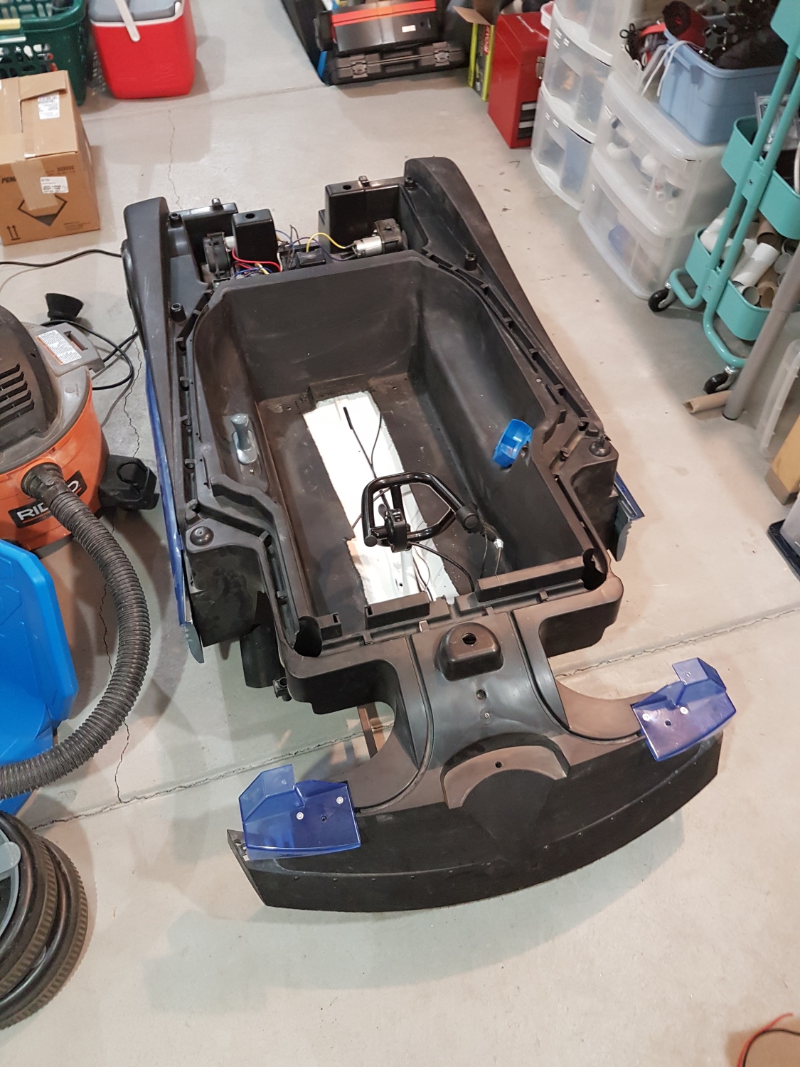
Seats? Where we’re going, we don’t need seats!

Pleasingly, the Batmobile sits on top of the chassis under its own structural support. We didn’t need to add all-thread or other standoffs. Even though they don’t do anything, we reattached the original wheels just so it looked extra wacky.

Motor and Motor Control

Moar!

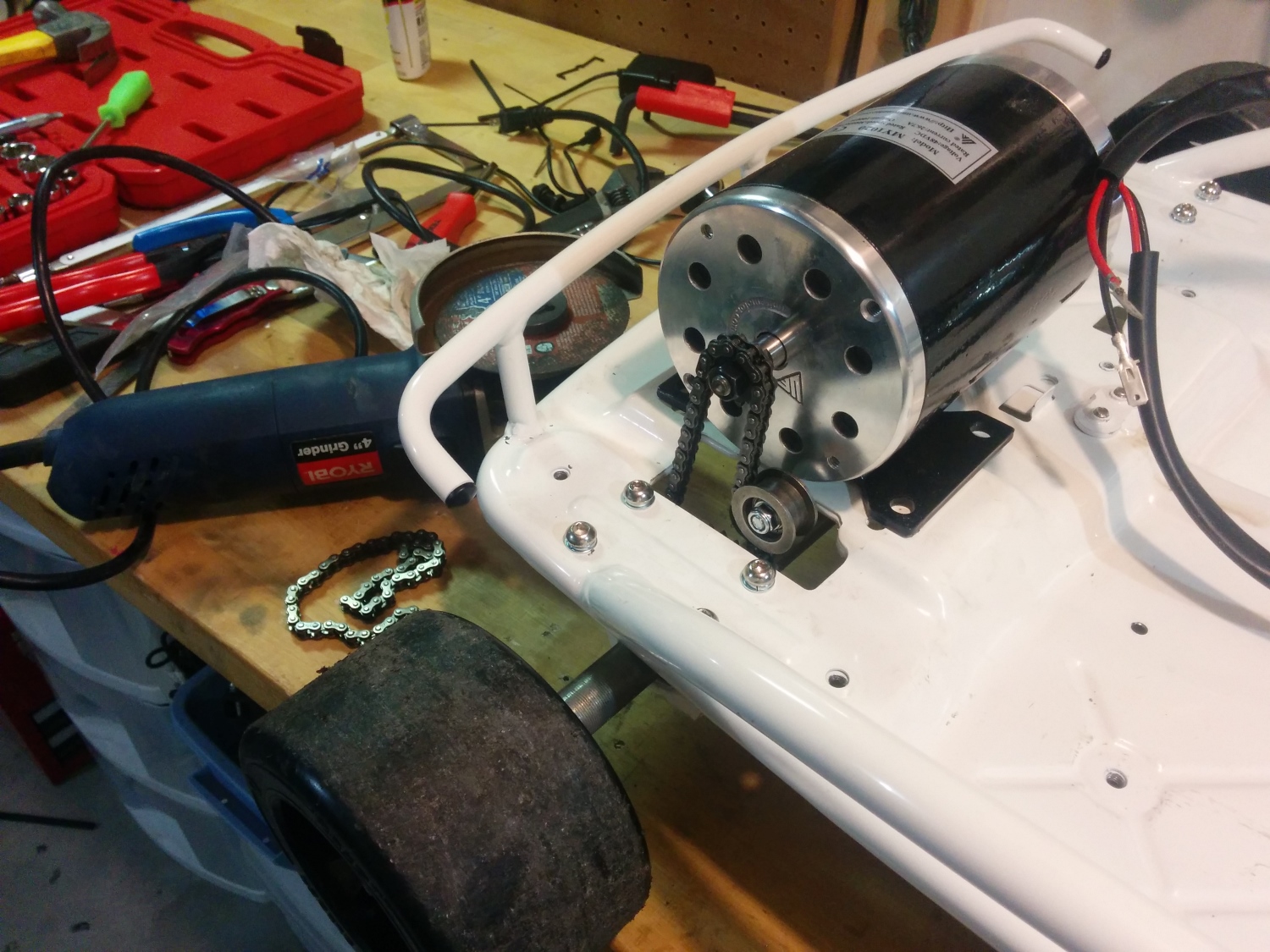
In 2016, A+PRS allowed 48V systems, so the first thing we did was remove the 24V motor and install a 1,000W 48V/21A motor. The PRS rules limit any system to 1,400W, so we could have gone larger had budget constraints not been kicking in fast. New mounting holes were drilled into the chassis, and a different gear had to be mounted to the end of the motor. But it all went well. The stock chassis even included a chain tensioner that proved invaluable!

The MY1020 48V motor we used is common on the PRS circuit and performed great. However, our original 1,000W motor controller (you should already be able to tell what’s coming) did not do so well. Our first tests of the 48V system in an open parking lot worked great until the motor controller overheated and failed. And when MOSFET-based motor controllers fail, they fail unsafe, meaning our vehicle decided to go to 100 percent throttle and stay there. This is why we have safety switches! Alicia and I were able to kill the vehicle before anyone got hurt.

This failure should have been prevented: a motor controller should be rated for at least 2 times what you calculate your maximum load will be. In our case, if we wanted to control a 1kW motor, we should have been using a motor controller rated to a constant 2kW load. Luckily, the A+PRS rules don’t require you to record how much money you spent (and burned up); you have to report only what is on the vehicle as it rolls on race day.

The new, larger 5kW motor controller

We quickly located a larger, 5kW motor controller (this one even had reverse!) and got it on order. This larger motor controller has been working swimmingly ever since. Find a motor controller with reverse. You’ll be tempted to drive your souped-up Power Wheels in weird places (like the SparkFun inventory aisles), and a reverse gear allows for hilarious 5-point turns.

Brakes

Go-kart drum brakes on eBay

The Razor chassis had the classic drum brake, perhaps the weakest link of the Razor. While the stock brake was probably the appropriate size for a 75lb child with stock 24V batteries, our brakes got really squishy once we added an additional 125lbs of meat bag, batteries and plastic bits. We rarely, if ever, used the brakes during races, but the PRS rules stipulate that your qualifying lap must end with the driver crossing the finish line and braking to a stop:

At the end of the hot lap, your car will have to come to a complete stop within 18ft of when its transponder crossed the start/finish line. Deliberately skidding, swerving or spinning out is not an acceptable method of braking for the brake test.

Alicia had to do an impressive combination of hard braking, swerving, skidding and sliding with such a dramatic flair that she wooed the judges into not noticing how dodgy our brakes were. We’ll have disc brakes installed before we roll in the 2017 race.

Batteries

Battery holder welded onto the front of the chassis

As part of the motor upgrade, we needed to increase the battery voltage to 48V. To save money, we reused the super common batteries that came with the 24V Razor chassis. Razor was smart; they looked at the SLA (Sealed Lead Acid) battery industry and picked the most common size. This just happened to be the same battery that goes into nearly every UPS on the planet. We purchased two additional UPS-size batteries (way cheaper than buying Razor-brand batteries) and wired them in series.

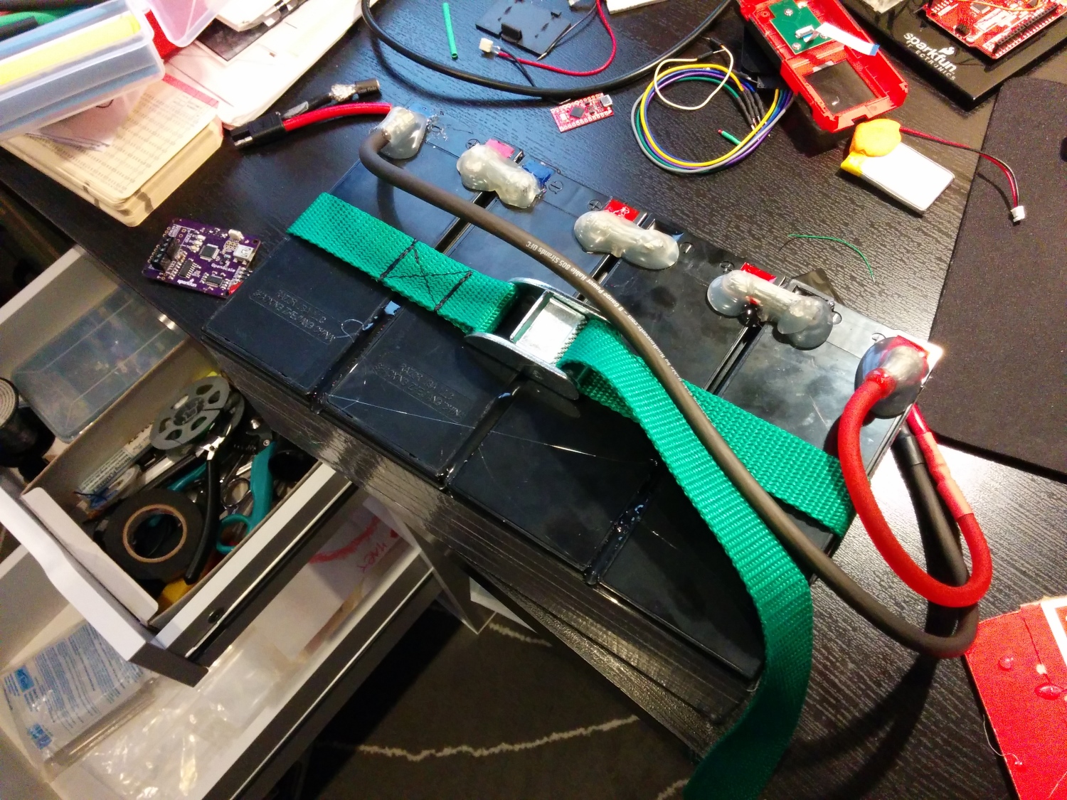
Four batteries combined in series

Taping the cells together and adding a bead of hot glue between the cells made the pack nicely rigid. A low-cost, polarized, high-current connector finished off the pack. We had an old strap lying around that made all the difference in the world; it’s a lot more comfortable carrying the pack one-handed by its handle than with two hands underneath.

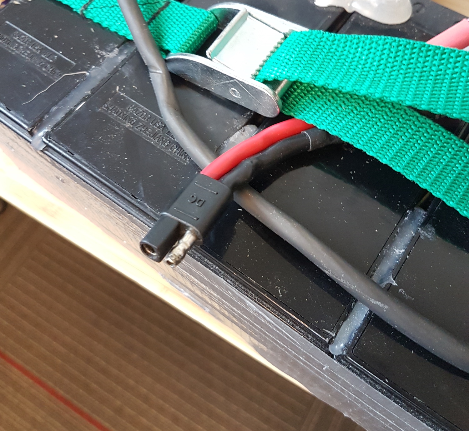
Avoid fires and other bad things. Use polarized connectors for your batteries.

Wire

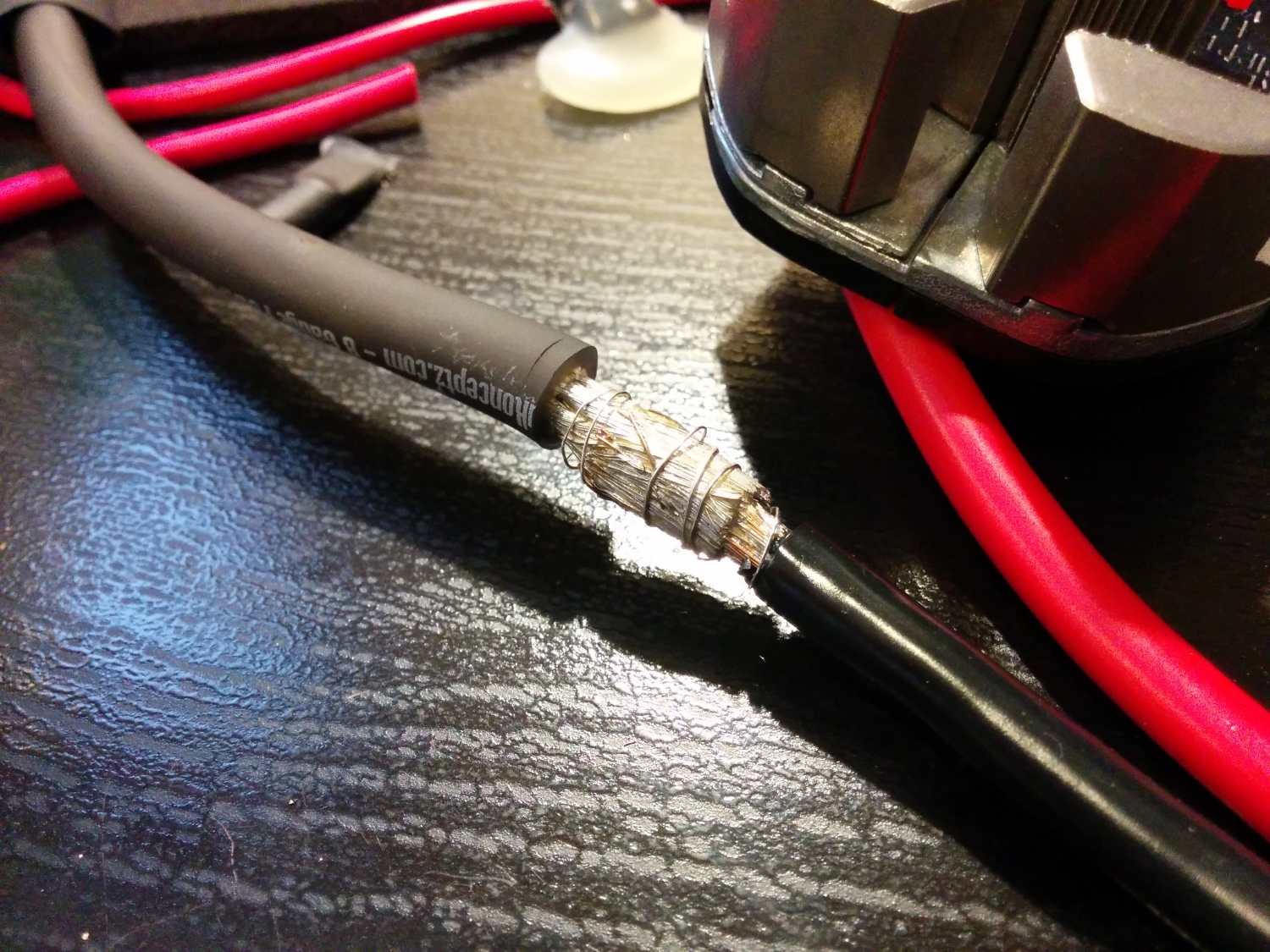
Soldering large-gauge wire

We originally spec’d out some really nice, super flexible silicone-sheathed 8AWG wire for power distribution. I don’t think we would do this again; 10AWG would have been fine, and probably even 12AWG. As 8-gauge is far less common, the wire and connectors are more expensive, and the larger gauge wire takes a lot more soldering heat — it’s just a pain to work with. If you need the current capacity, go for it, but for our extremely zippy, 48V 20A vehicle, 8-gauge wire was overkill.

If you decide to use super flexible, large gauge wire, spend some time on the internet reading about how to solder this type of wire.

The best technique I found:

Make sure you’ve got heat shrink in place
Turn your soldering iron up to 425C (way hotter than the 325C usually needed)
Push the ends of wire together
Wrap tightly with 30AWG wire wrap wire
Liberally apply flux
Heat and insert lots of solder until the joint turns silver

Here’s a good video demonstrating this technique:

Kill Switch

We documented how to build a wireless kill switch while making margaritas. It was a ton of fun, so we’ll skip the bits of the wireless kill switch system here.

Zroooommmm!

In addition to the wireless disconnect, we had a large, red mushroom kill switch that disconnected the battery with a pleasing and authoritative ”thunk.” Pulling up on the mushroom button reconnects the battery to the system.

Batman logo or Bitman logo?

As a pleasant bonus feature, the mushroom kill switch got rid of the nasty sparks. When connecting the battery to the motor controller, there was such an inrush of current into the capacitors and electronics that the connector would spark. Once we got the kill switch installed, we could connect/disconnect batteries without these sparks.

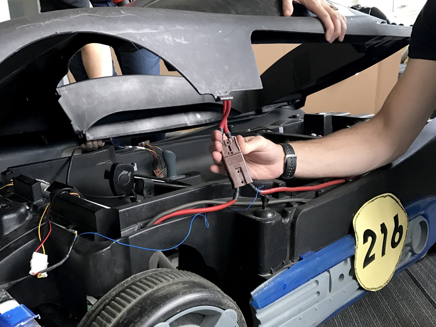
Connector between kill switch and power bus

The top of the Batmobile was easily removed, but because it had the kill switch installed we needed a way to disconnect it easily from the power bus. We found a great high-power connector in a dead server UPS. These are often called ”winch connectors”, because they are higher current. With this connector, we are able to quickly disconnect the kill switch and remove the top when we need to get at the inside of the vehicle.

Control Electronics

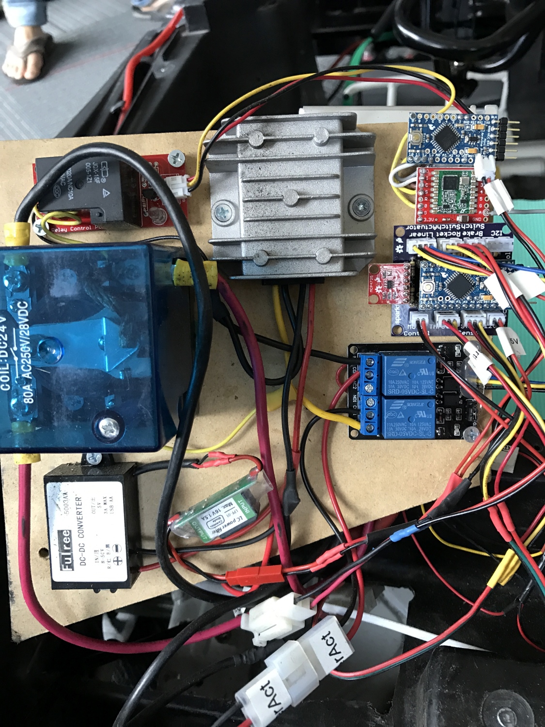
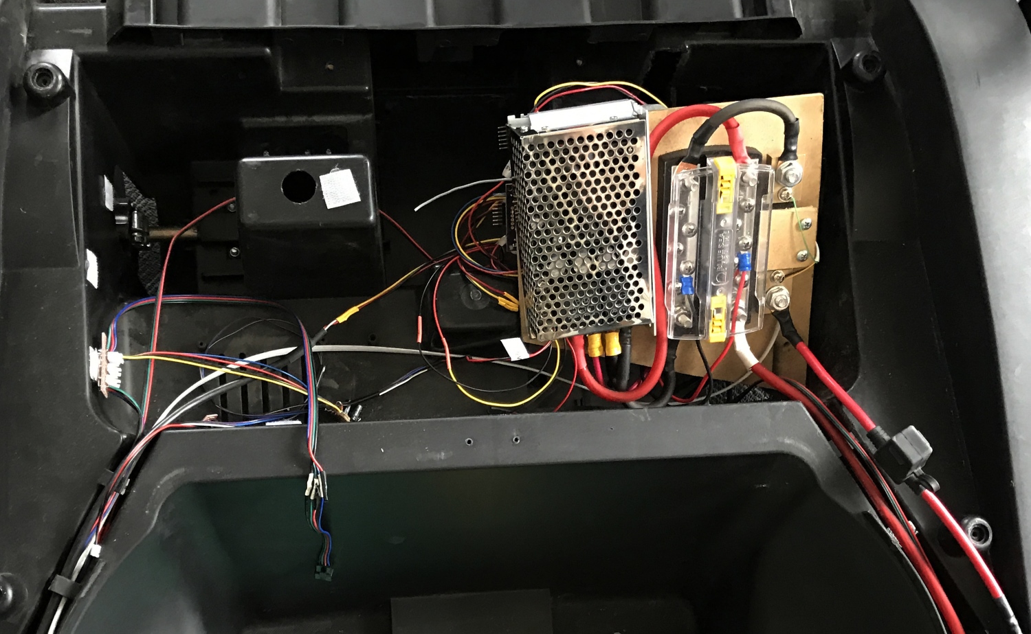
Power converters, motor kill relays, steering relays, locomotion controller and wireless communication

The control electronics are complex. We had a total of seven microcontrollers on this beast, plus three used in the distance sensors for a total of 216 bits of processing power. The system operated on an I²C bus with the brain sending commands to the locomotion controller and LCD and receiving data from the sensors.

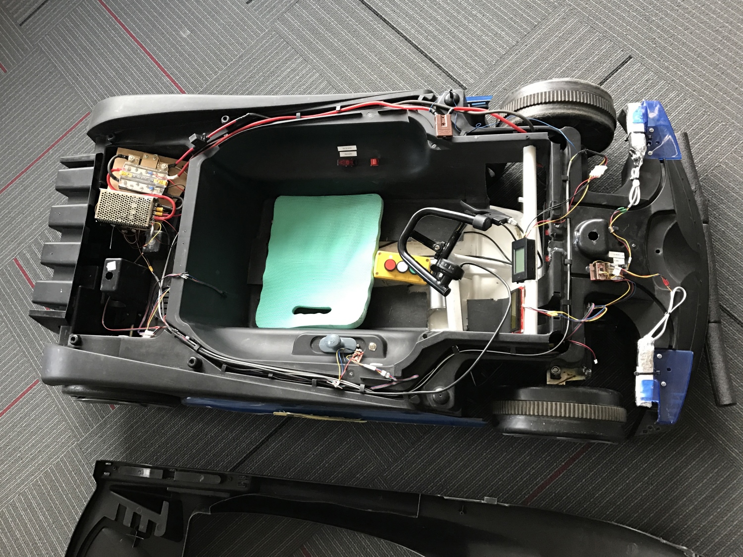
The wiring underneath the Batmobile cover

For a previous 2010 AVC entry, I did everything on a single microcontroller. This made coding and debugging a challenge. On our 2016 entry, we focused each sub-system to do one thing very well.

The subsystems are broken down as follows:

Brain Controller: A SAMD21 Mini was used to communicate with and process all the data from the distance sensors, GPS and compass, and to send out commands to control throttle and steering. It monitored a start switch and relayed debug information to an LCD.
Locomotion Controller: An Arduino Pro Mini read the throttle, steering position, brake switch and autonomous rocket switch. It controlled motor speed and the linear actuator for steering.
Wireless Kill Switch: An Arduino Pro Mini lived in the wireless kill switch, a requirement for the autonomous part of our Batmobile. To learn more about the wireless controller, check out our tutorial on how to build a wireless kill switch.
A dedicated Arduino Pro Mini controlled the relays for the wireless kill switch system.
Debug LCD: We counted our LCD screen as a microcontroller since it has an Arduino in it.
Sensor Combinator: A SAMD21 Mini polled the serial GPS and I²C compass.
Laser Controller: A SAMD21 Mini controlled the three serial-based laser distance sensors, combined the relevant information and responded to requests from the Brain.
Three STM32s were the brains within the laser distance sensors.

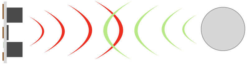
Interested in learning more about distance sensing?

Learn all about the different technologies distance sensors use and which products would work best for you next project.TAKE ME THERE!

Control Electronics – Brain

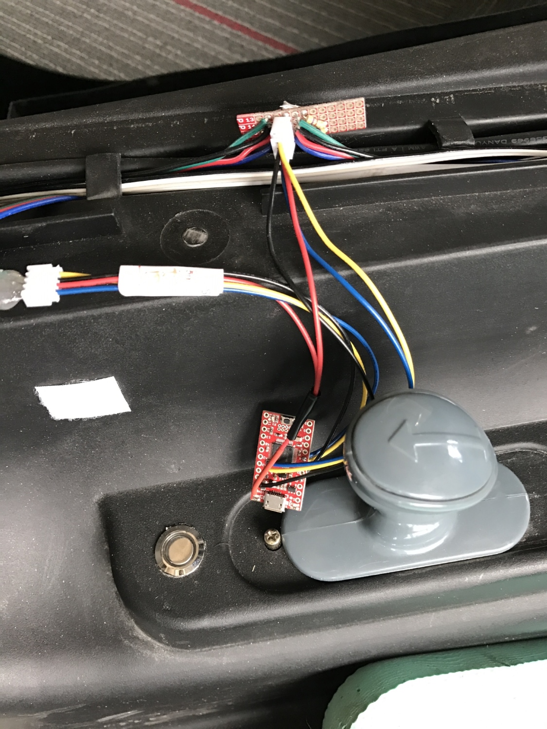
The Brain is a SAMD21 Mini. It sends commands over the I²C bus to the locomotion controller and debug LCD.

4-pin JST connector at the top of the image: We used a 4-wire bus (5V, GND, SDA, SCL) for communication and had various taps throughout the bus to allow devices to be attached. This worked really well and allowed for devices to be moved around when needed.

4-pin JST connector to the left: This was four wires to the button. To tell the vehicle to begin navigating under autonomous control, we used a metal momentary push button that illuminates when everything is online and happy. The human presses the button twice, and the car commences racing.

Big gray handle: This was the original forward and reverse knob that we reused to control the direction switch on the motor controller (two pins when shorted together caused one direction, when open caused the other direction).

The massive and poorly written control code for the Brain can be found here.

EEPROM for Waypoints

The SAMD21 does not have internal EEPROM. Because we needed to store GPS waypoints and other configuration data to non-volatile memory, we used an external I²C EEPROM. Yes, you can use something called emulated EEPROM on the SAMD21, but, every time you reprogram the board, you will overwrite anything previously stored in emulated EEPROM. The external EEPROM made it much easier to store and recall waypoints and settings without having to mash together in the main control code.

Control Electronics – Locomotion

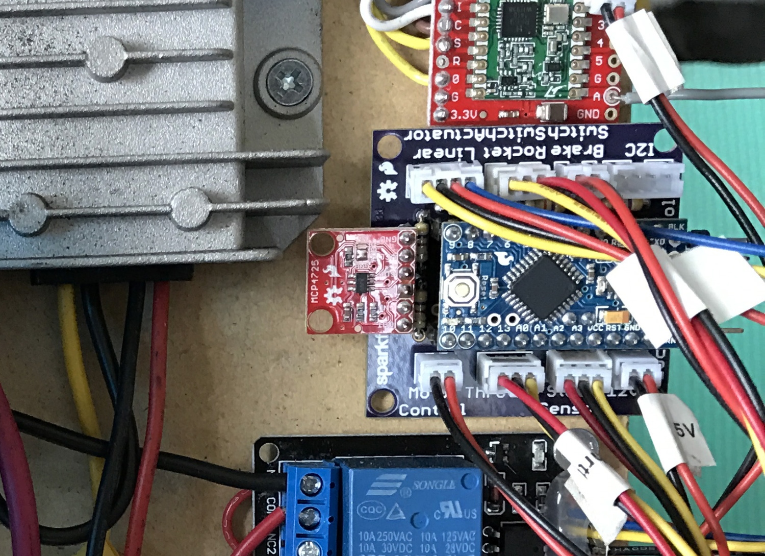
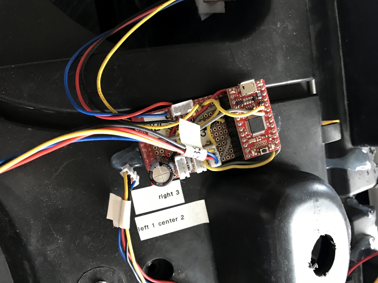
Locomotion Controller hooked up

Note the polarized connectors and prodigious labeling! You DO NOT want to be guessing what gets plugged into where at 11 p.m. before race day. The Locomotion Controller code is available here, and the PCB layout here.

Because we eventually wanted this beast to be autonomous, we needed to put a controller in the middle between the throttle and the motor controller. We used an Arduino Pro Mini that did a huge variety of sensing and control:

Read the throttle
Output analog voltage to the motor controller
Read the brake switch
Read the steering position
Controlled the linear steering actuator
Read the human/robot control switch
Received and responded to control commands over I²C

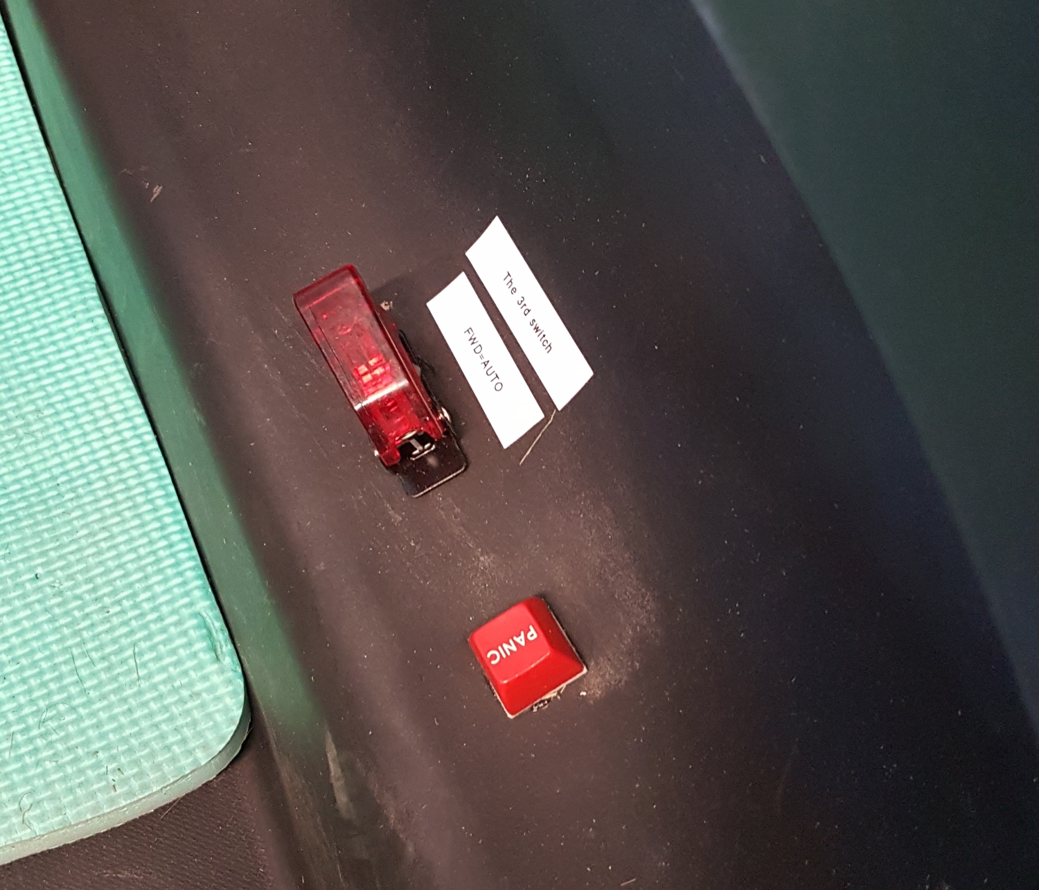
Don’t panic

The controller would monitor the rocket switch and brake switch. If a human ever pressed the brakes or turned off the rocket switch, the controller would go into safety shutdown and ignore any commands from the brain.

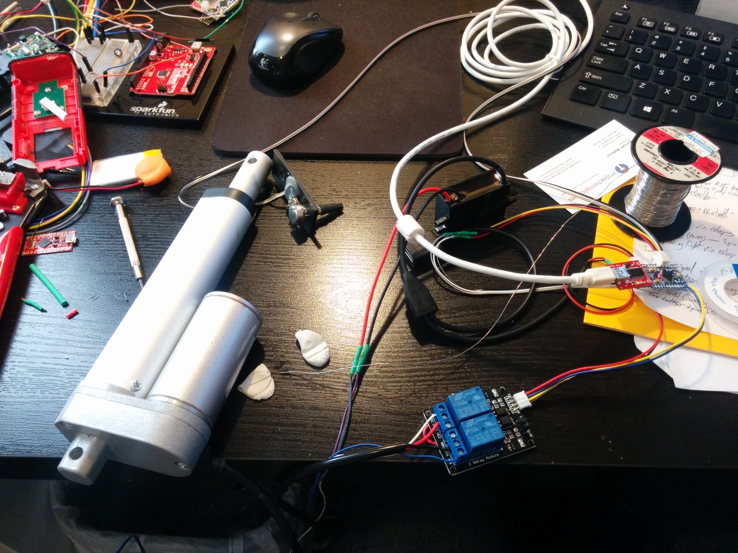
Steering was controlled using a 12V linear actuator over-voltaged to 24V for extra speed. Two relays controlled the forward/backward motion.

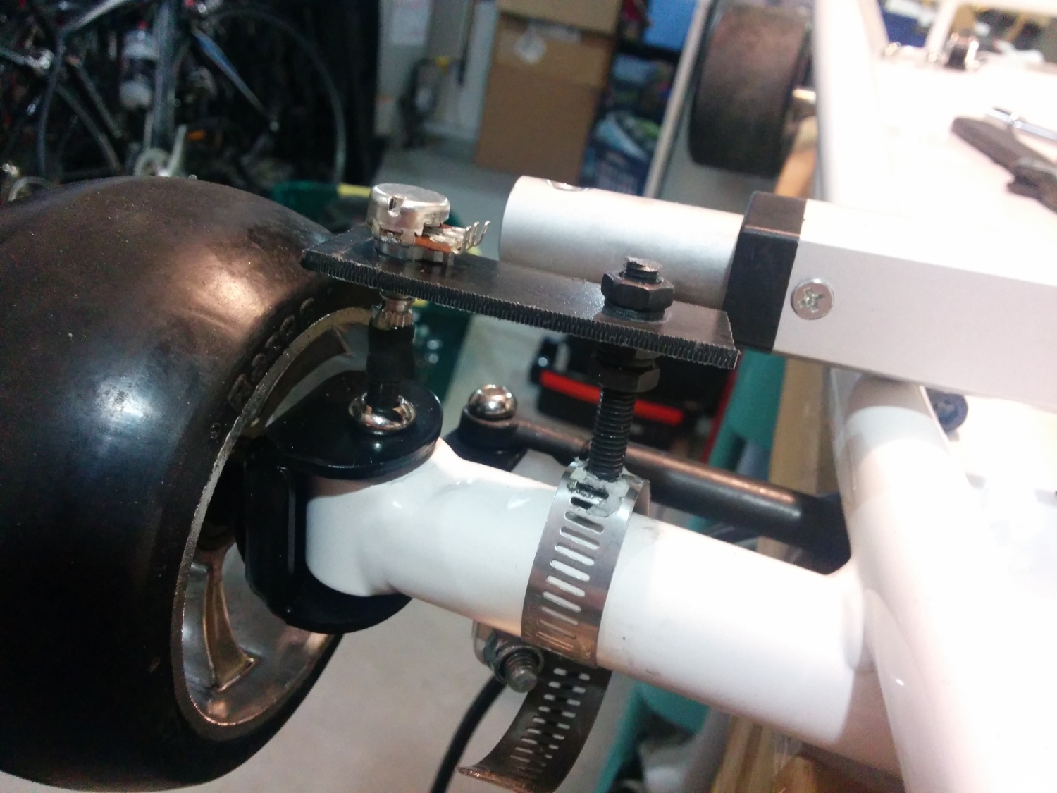
Steering position was obtained by cutting a hex wrench to about 1” and inserting that wrench into the bolt that rotates with the wheel. The wrench was then connected to a 10k trimpot using adhesive-lined heat shrink — this trick is known as the ”poor man’s coupler:” a 3-wire ribbon connected the trimpot back to the locomotion controller. It worked well, but we had to keep the analog signal wire away from the power bus; otherwise, bad noise got into the ADC readings.

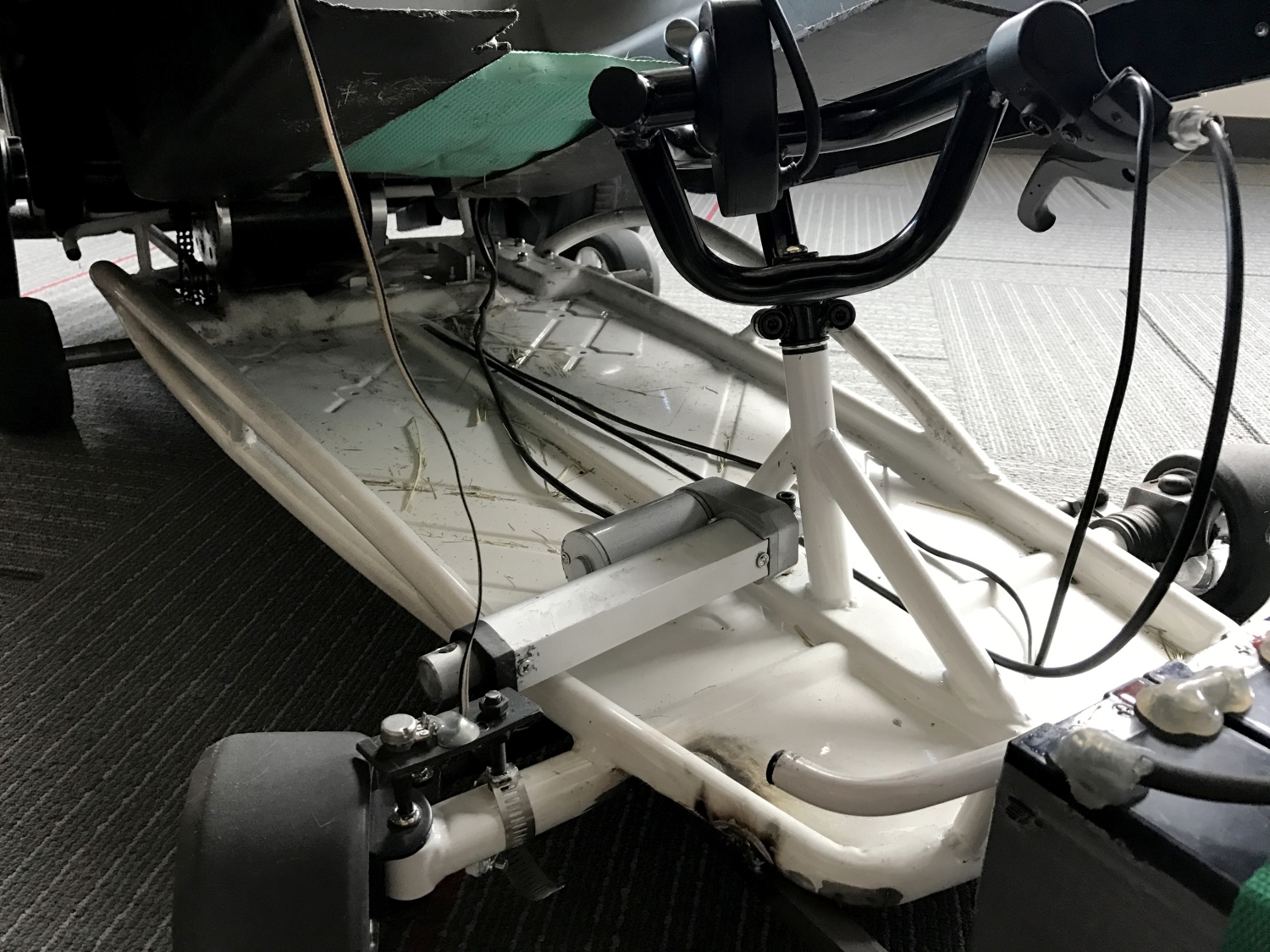
Chassis with the Batmobile raised to see the steering actuator

For future vehicles, we’re going to change this setup. It worked well enough, but once the bolt connected the actuator to the steering, you couldn’t drive the car; only the computer could. So rather than driving the car to the start line, we had to carry this 75lb beast. So painful. In the future, we plan to find a back-drivable actuator or maybe drive-by-wire.

Control Electronics – Displays

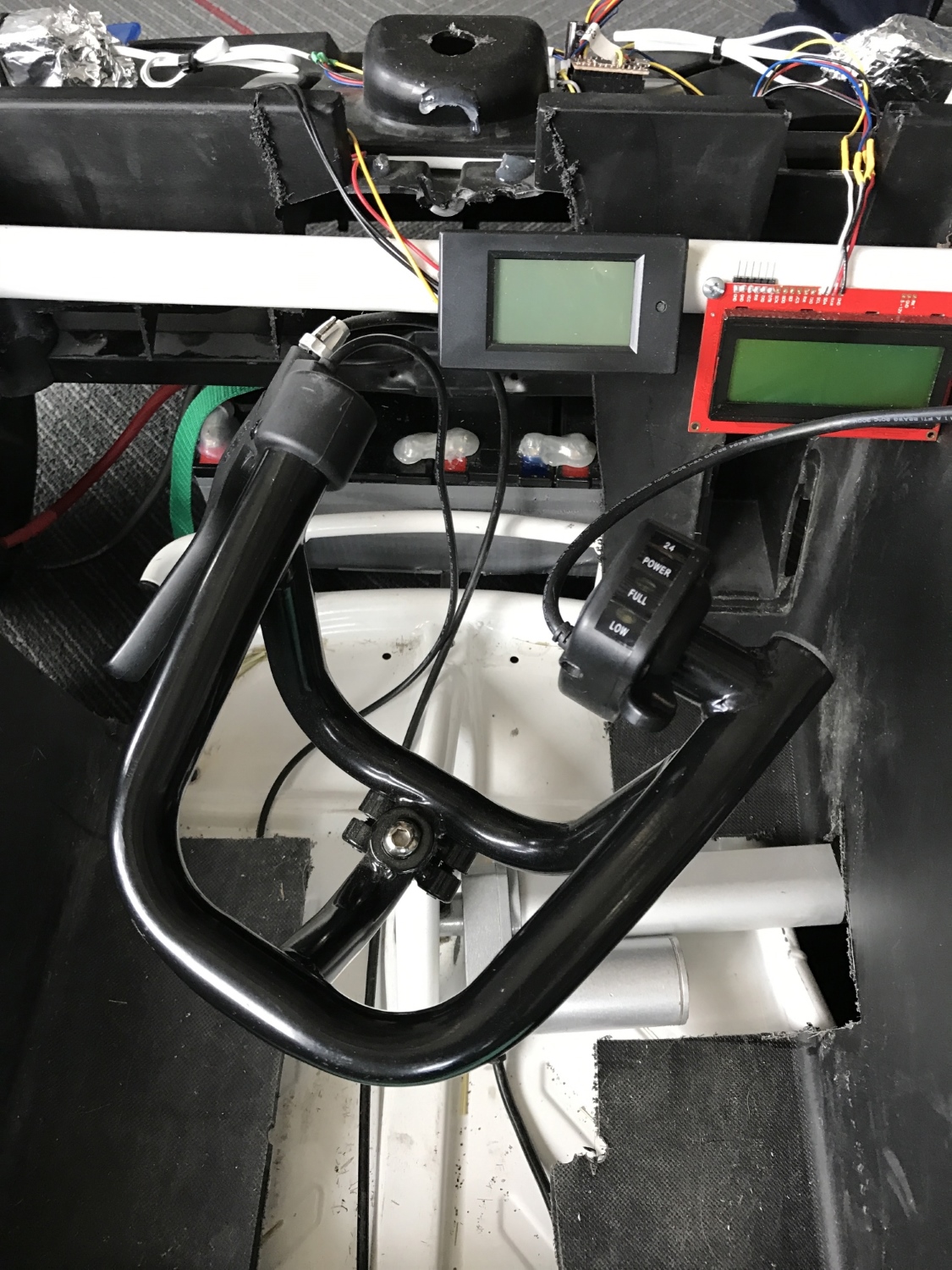
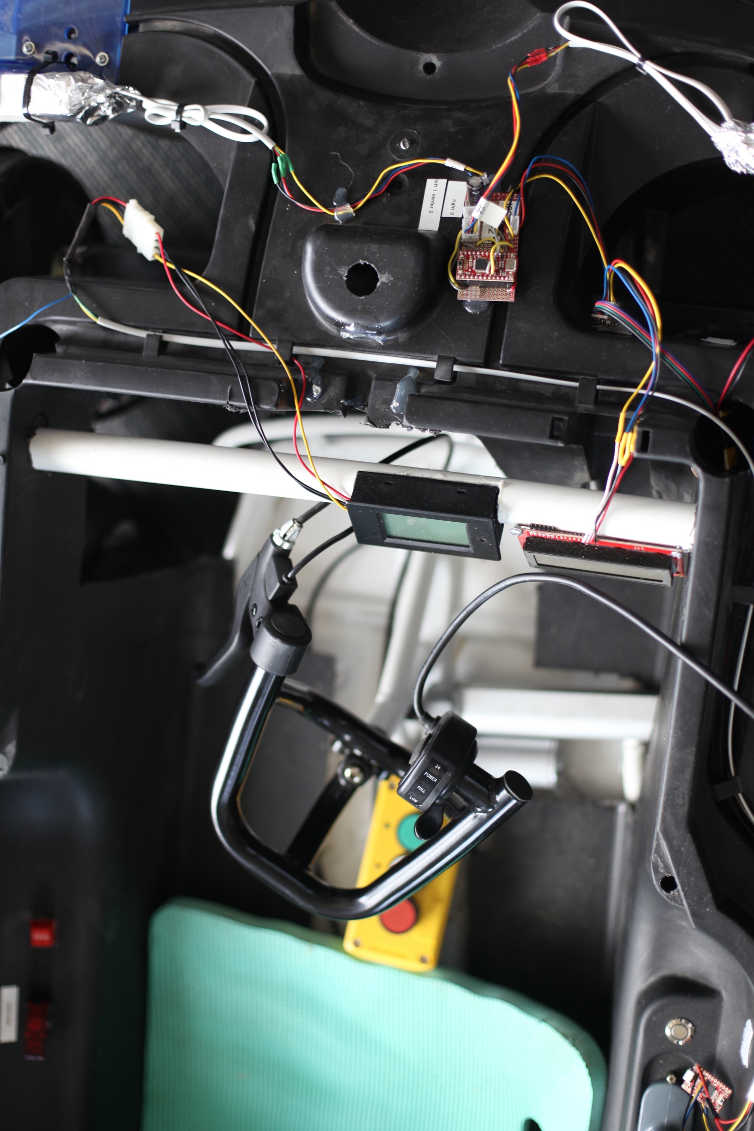
Throttle and displays

We cut notches in a 1” tube of PVC and mounted two displays in the Batmobile. The center display is the power meter. Nearly every A+PRS and PRS competitor used these super low-cost power meters to show the battery voltage. We had some issues with it, but it worked well enough. In the end, we noticed the drop in vehicle speed (indicating battery drain) long before we noticed the display was indicating a lower pack voltage. But, it did help us make decisions about when to pit (never!) because the nominal 48V pack voltage was dropping down to 42V where we could begin to damage the SLA.

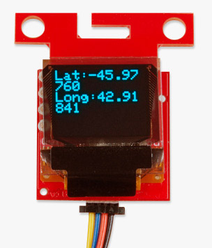
The display on the right is the 20×4 character debug LCD. It’s basically a souped-up version of our 20×4 SerLCD display (it’s a prototype product, coming soon to a theater near you!).

Control Electronics – Sensors

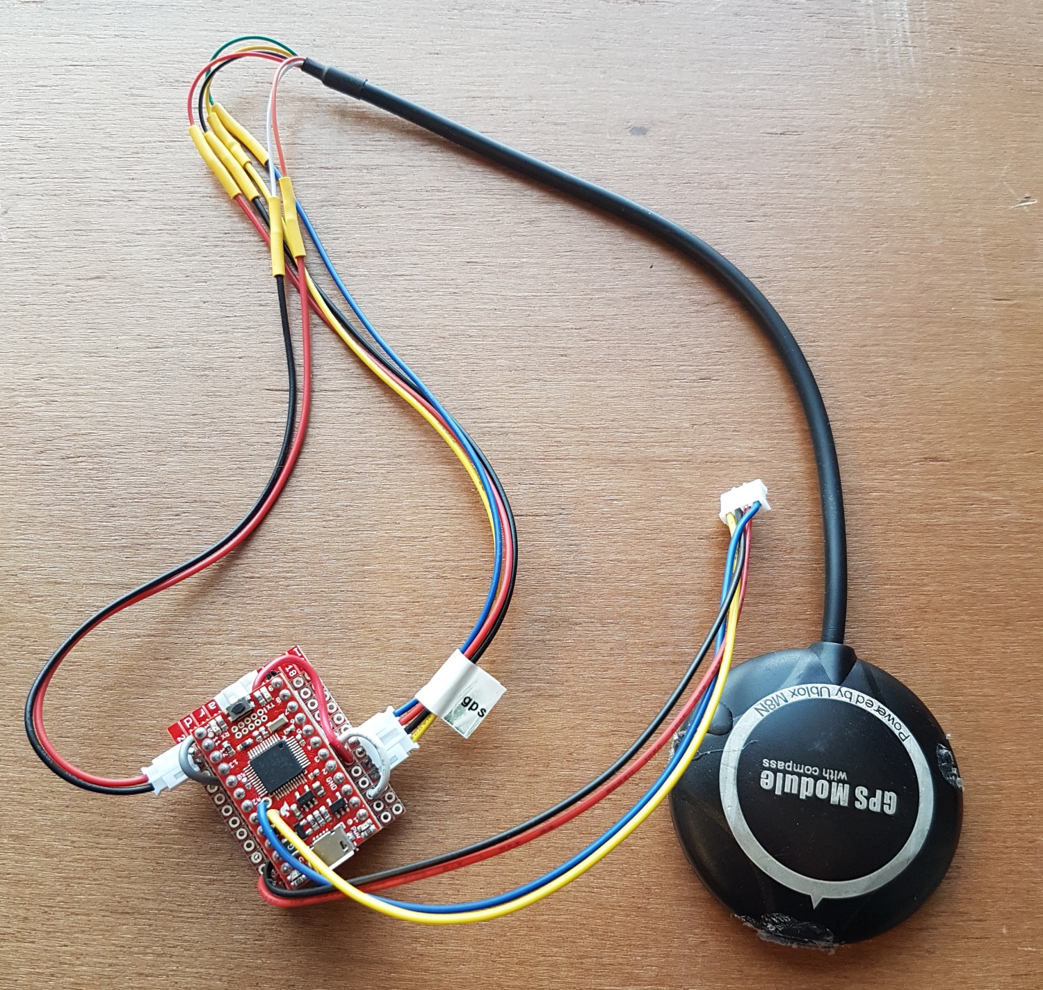
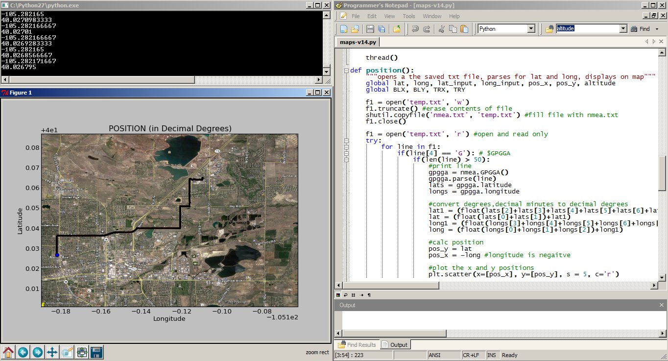
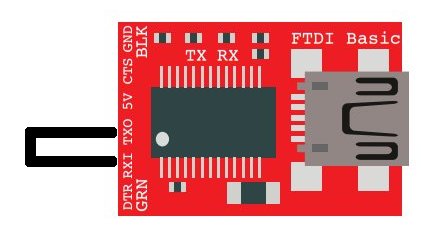
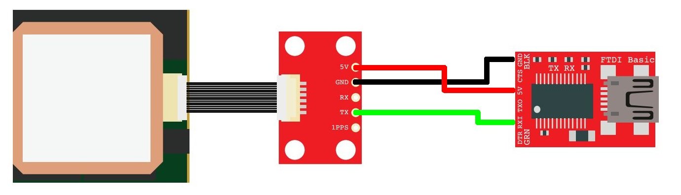
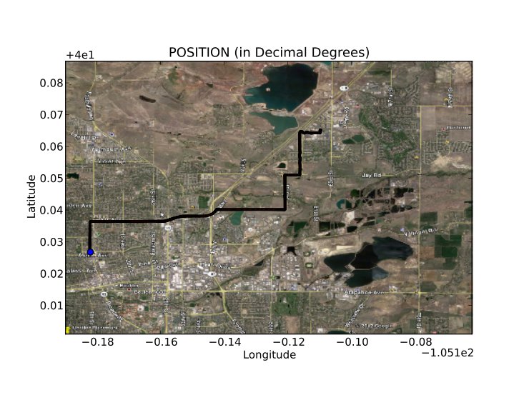
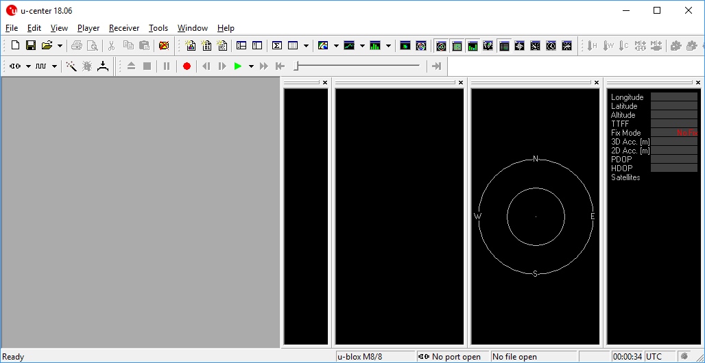
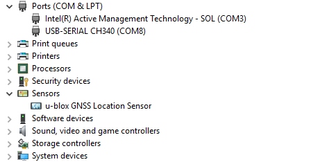
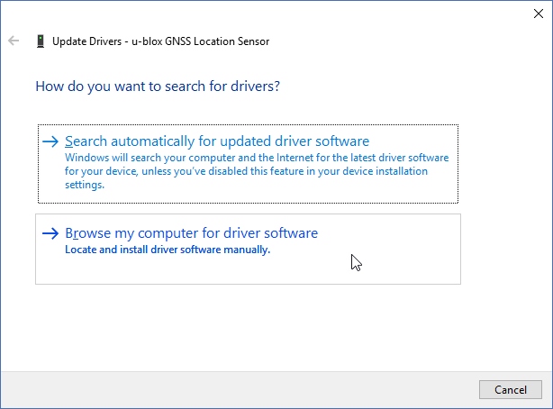
GPS+Compass connected to SAMD21

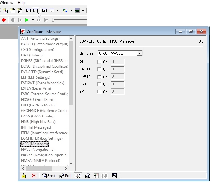
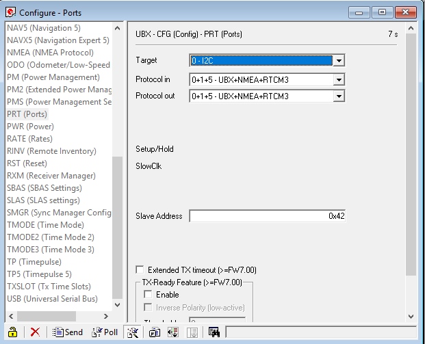
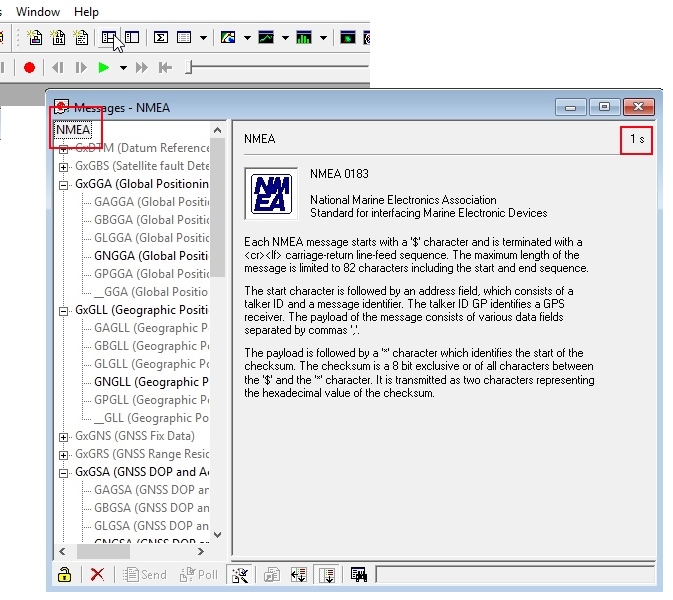
The Sensor Combinator is a SAMD21 Mini that monitors a GPS receiver and an I²C compass. We decided to use a SAMD21 because it can be configured to have multiple hardware serial and I²C ports. This is needed if you want to isolate I²C devices from the main bus. We wanted the Brain to ask for the heading and get the heading; the Sensor Combinator took care of the low-level I²C function of the compass and heading calculations. Similarly, the Combinator listened to the serial stream from the u-blox based GPS module and parsed out all the needed Latitude/Longitude/SIV information.

The code for the Sensor Combinator can be found here.

Control Electronics – Lasers

Laser tape measures seen on the front of the car, wrapped in foil

We hacked three laser tape measures in order to get distance to any objection front, left or right of the car. Laser tape measures are getting cheaper, and while the read rate (3Hz at the best of times) is not great for LIDAR, it’s fast enough for basic, low-cost autonomy.

Laser Controller at front of car

Unfortunately, the laser tape measures threw off enough RF to interfere with our GPS module, so we wrapped the lasers in foil. These sensors deserve their own tutorial, which will be written soon.

Laser Controller with labels

Again we chose the SAMD21 Mini to help us control and combine the serial information coming from the three sensors. The Laser Controller would send the pertinent control strings to the tape measures and monitor the responses, combining them into distances for left/right/center. The Brain would request these values from the Laser Controller over I²C.

Note the prodigious amounts of labels and polarized connectors (JSTs work great!). This system required lots of debugging but worked well because we were able to quickly disconnect and reconnect various aspects of the system.

The code for the Laser Controller can be found here.

Problems

As with any project, we had a large number of problems and hurdles to overcome along the way. Here are a few that really hurt.

** EMI and GPS **

The Laser tape measures caused significant interference with GPS reception. We eventually moved the GPS module to the rear of the car, which improved positional accuracy. However, the motor caused interference with the compass.

** DC Motor EMF **

DC motors produce a ton of electromagnetic noise. We originally had the 48V battery powering the entire car. However, when the motor would kick on, it would cause enough ripple to make the Brain glitch and reset. We tried powering the I²C bus separately, but, because the Locomotion Controller needed to be attached to the motor controller, a GND connection had to be shared. The noise eventually found its way over the I²C bus. In the future we will optically isolate the I²C bus.

** Lack of EEPROM **

Because the SAMD21 doesn’t have internal EEPROM, we were unable to store GPS waypoints on the board. We fixed this by using an I²C-based EEPROM.

** Switching Steering Between Driver/Driverless **

It was difficult to attach and detach the linear actuator from the rack and pinion steering. Once the actuator was attached to the steering, a driver could not actively steer (for example, to the starting line). This could be fixed with a different actuator that could be back-driven, or we could go full monty and detach the steering column from the steering and have it control a trimpot that, in turn, controls the linear actuator (drive by wire).

Tips / Best Practices

Tip 1) Start early — These vehicles take a large amount of time. Get together with friends and start hacking. It’s a great labor of love, and drifting in a 15mph go-kart will make you giggle.

Tip 2) Get reverse — Get a motor controller with reverse. It will make it so you can drive your car where you want it instead of carrying your car where you need it.

Tip 3) Use connectors! — I’ve written about using connectors a few times. Use polarized connectors and a label maker to make it clear what plugs in where.

Tip 4) Size your motor and motor controller correctly — We blew our motor controller because it was underrated. A friend of ours smoked his motor because he was pushing too much current. Pick your system voltage and current, and then double the ratings wherever you can.

Tip 5) Beware of interference — These vehicles can pull 30 amps or more when accelerating, which can cause large electromagnetic fields. Keep unshielded cables and sensitive sensors away from power wires.

Tip 6) Wireless control and sensor logging — After you pick up your 75lb vehicle and drag it to the start line for the fifth time, you’ll understand the need for remote control. Create a wireless system that allows you to take over control of the vehicle from afar so you can drive it where you need it. And transmit the sensor data so you can see what the vehicle is doing.

Python och GPS-spårning

Detta är en artikel från SparkFun, December 17, 2012

Introduction

In my quest to design a radio tracking system for my next HAB, I found it very easy to create applications on my computer and interact with embedded hardware over a serial port using the Python programming language. My goal was to have my HAB transmit GPS data (as well as other sensor data) over RF, to a base station, and graphically display position and altitude on a map. My base station is a radio receiver connected to my laptop over a serial to USB connection. However, in this tutorial, instead of using radios, we will use a GPS tethered to your computer over USB, as a proof of concept.

Of course, with an internet connection, I could easily load my waypoints into many different online tools to view my position on a map, but I didn’t want to rely on internet coverage. I wanted the position of the balloon plotted on my own map, so that I could actively track, without the need for internet or paper maps. The program can also be used as a general purpose NMEA parser, that will plot positions on a map of your choice. Just enter your NMEA data into a text file and the program will do the rest.

Showing a trip from SparkFun to Boulder, CO.

This tutorial will start with a general introduction to Python and Python programming. Once you can run a simple Python script, we move to an example that shows you how to perform a serial loop back test, by creating a stripped down serial terminal program. The loopback test demonstrates how to send and receive serial data through Python, which is the first step to interacting with all kinds of embedded hardware over the serial port. We will finish with a real-world example that takes GPS data over the serial port and plots position overlaid on a scaled map of your choice. If you want to follow along with everything in this tutorial, there are a few pieces of hardware you will need.

5V FTDI Basic
EM-406 GPS module with Breakout Board (or any NMEA capable GPS)

For the loopback test, all you need is the FTDI Basic. For the GPS tracking example, you will need a GPS unit, as well as the FTDI.

What is Python?

If you are already familiar with installing and running Python, feel free to skip ahead. Python is an interpreted programming language, which is slightly different than something like Arduino or programming in C. The program you write isn’t compiled as a whole, into machine code, rather each line of the program is sequentially fed into something called a Python interpreter. Once you get the Python interpreter installed, you can write scripts using any text editor. Your program is run by simply calling your Python script and, line by line, your code is fed into the interpreter. If your code has a mistake, the interpreter will stop at that line and give you an error code, along with the line number of the error.

The holy grail for Python 2.7 reference can be found here:

python.org

Installing Python

At the time of this tutorial, Python 2.7 is the most widely used version of Python and has the most compatible libraries (aka modules). Python 3 is available, but I suggest sticking with 2.7, if you want the greatest compatibility.

Download and Install Python 2.7

After you install Python, you should be able to open a command prompt within any directory and type ’python’. You should see the interpreter fire up.

If you don’t see this, it is time to start some detective work. Copy your error code, enter it into your search engine along with the name ’python’ and your OS name, and then you should see a wealth of solutions to issues similar, if not exact, to yours. Very likely, if the command ’python’ is not found, you will need to edit your PATH variables. More information on this can be found here. FYI, be VERY careful editing PATH variables. If you don’t do it correctly, you can really mess up your computer, so follow the instructions exactly. You have been warned.

If you don’t want to edit PATH variables, you can always run Python.exe directly out of your Python installation folder.

Running a Python Script

Once you can invoke the Python interpreter, you can now run a simple test script. Now is a good time to choose a text editor, preferably one that knows you are writing Python code. In Windows, I suggest Programmers Notepad, and in Mac/Linux I use gedit. One of the main rules you need to follow when writing Python code is that code chunks are not enclosed by brackets {}, like they are in C programming. Instead, Python uses tabs to separate code blocks, specifically 4 space tabs. If you don’t use 4 space tabs or don’t use an editor that tabs correctly, you could get errant formatting, the interpreter will throw errors, and you will no doubt have a bad time.

For example, here is a simple script that will print ’test’ continuously.

# simple script
def test():
    print "test"
while 1:
    test()

Now save this code in a text editor with the extention your_script_name.py.

The first line is a comment (text that isn’t executed) and can be created by using a # .

The second line is a function definition named test().

The third line is spaced 4 times and is the function body, which just prints ”test” to the command window.

The third line is where the code starts in a while loop, running the test() function.

To run this script, copy and paste the code into a file and save it with the extention .py. Now open a command line in the directory of your script and type:

python your_script_name.py

The window should see the word ’test’ screaming by.

To stop the program, hit Ctrl+c or close the window.

Installing a Python Module

At some point in your development, you will want to use a library or module that someone else has written. There is a simple process of installing Python modules. The first one we want to install is pyserial.

pyserial

Download the tar.gz file and un-compress it to an accessible location. Open a command prompt in the location of the pyserial directory and send the command (use sudo if using linux):

python setup.py install

You should see a bunch of action in the command window and hopefully no errors. All this process is doing is moving some files into your main Python installation location, so that when you call the module in your script, Python knows where to find it. You can actually delete the module folder and tar.gz file when you are done, since the relevant source code was just copied to a location in your main Python directory. More information on how this works can be found here:

Installing Python Modules

FYI, many Python modules can be found in Windows .exe installation packages that allow you to forgo the above steps for a ’one-click’ installation. A good resource for Windows binary files for 32-bit and 64-bit OS can be found here:

http://www.lfd.uci.edu/~gohlke/pythonlibs/

Python Serial Loopback Test

This example requires using an FTDI Basic or any other serial COM port device.

Simply, connect the TX pin to the RX pin with a wire to form a loopback. Anything that gets sent out of the serial port transmit pin gets bounced back to the receive pin. This test proves your serial device works and that you can send and receive data.

Now, plug your FTDI Basic into your computer and find your COM port number. We can see a list of available ports by typing this:

python -m serial.tools.list_ports

If you are using linux:

dmesg | grep tty

Note your COM port number.

Now download the piece of code below and open it in a text editor (make sure everything is tabbed in 4 space intervals!!):

import serial

#####Global Variables######################################
#be sure to declare the variable as 'global var' in the fxn
ser = 0

#####FUNCTIONS#############################################
#initialize serial connection 
def init_serial():
    COMNUM = 9 #set you COM port # here
    global ser #must be declared in each fxn used
    ser = serial.Serial()
    ser.baudrate = 9600
    ser.port = COMNUM - 1 #starts at 0, so subtract 1
    #ser.port = '/dev/ttyUSB0' #uncomment for linux

    #you must specify a timeout (in seconds) so that the
    # serial port doesn't hang
    ser.timeout = 1
    ser.open() #open the serial port

    # print port open or closed
    if ser.isOpen():
        print 'Open: ' + ser.portstr
#####SETUP################################################
#this is a good spot to run your initializations 
init_serial()

#####MAIN LOOP############################################
while 1:
    #prints what is sent in on the serial port
    temp = raw_input('Type what you want to send, hit enter:\n\r')
    ser.write(temp) #write to the serial port
    bytes = ser.readline() #reads in bytes followed by a newline 
    print 'You sent: ' + bytes #print to the console
    break #jump out of loop 
#hit ctr-c to close python window

First thing you need to do before running this code is to change the COM port number to the one that is attached to your FTDI. The COMNUM variable in the first few lines is where you enter your COM port number. If you are running linux, read the comments above for ser.port.

Now, if you want to send data over the serial port, use:

ser.write(your_data)

your_data can be one byte or multiple bytes.

If you want to receive data over the serial port, use:

your_data = ser.readline()

The readline() function will read in a series of bytes terminated with a new line character (i.e. typing something then hitting enter on your keyboard). This works great with GPS, because each GPS NMEA sentence is terminated with a newline. For more information on how to use pyserial, look here.

You might realize that there are three communication channels being used:

ser.write – writes or transmitts data out of the serial port
ser.read – reads or receives data from the serial port
print – prints to the console window

Just be aware that ’print’ does not mean print out to the serial port, it prints to the console window.

Notice, we don’t define the type of variables (i.e. int i = 0). This is because Python treats all variables like strings, which makes parsing text/data very easy. If you need to make calculations, you will need to type cast your variables as floats. An example of this is in the GPS tracking section below.

Now try to run the script by typing (remember you need to be working out of the directory of the pythonGPS.py file):

python pythonGPS.py

This script will open a port and display the port number, then wait for you to enter a string followed by the enter key. If the loopback was successful, you should see what you sent and the program should end with a Python prompt >>>.

To close the window after successfully running, hit Ctrl + c.

Congratulations! You have just made yourself a very simple serial terminal program that can transmit and receive data!

Read a GPS and plot position with Python

Now that we know how to run a python script and open a serial port, there are many things you can do to create computer applications that communicate with embedded hardware. In this example, I am going to show you a program that reads GPS data over a serial port, saves the data to a txt file; then the data is read from the txt file, parsed, and plotted on a map.

There are a few steps that need to be followed in order for this program to work.Install the modules in the order below.

Install modules

Use the same module installation process as above or find an executable package.

pyserial (should already be installed from above)
numpy (use: this link for Windows and this link for Mac/Linux)
matplotlib
pynmea

The above process worked for me on my W7 machine, but I had to do some extra steps to get it to work on Ubuntu. Same might be said about Macs. With Ubuntu, you will need to completely clean your system of numpy, then build the source for numpy and matplotlib separately, so that you don’t mess up all of the dependencies. Here is the process I used for Ubuntu.

Once you have all of these modules installed without errors, you can download my project from github and run the program with a pre-loaded map and GPS NMEA data to see how it works:

github-gps_tracker

Or you can proceed and create your own map and GPS NMEA data.

Select a map

Any map image will work, all you need to know are the bottom left and top right coordinates of the image. The map I used was a screen shot from Google Earth. I set placemarks at each corner and noted the latitude and longitude of each corner. Be sure to use decimal degrees coordinates.

Then I cropped the image around the two points using gimp. The more accurate you crop the image the more accurate your tracking will be. Save the image as ’map.png’ and keep it to the side for now.

Hardware Setup

The hardware for this example includes a FTDI Basic and any NMEA capable GPS unit.

EM-406 GPS connected to a FTDI Basic

For the connections, all you need to do is power the GPS with the FTDI basic (3.3V or 5V and GND), then connect the TX pin of the GPS to the RX pin on the FTDI Basic.

It is probably best to allow the GPS to get a lock by leaving it powered for a few minutes before running the program. If the GPS doesn’t have a lock when you run the program, the maps will not be generated and you will see the raw NMEA data streaming in the console window. If you don’t have a GPS connected and you try to run the program, you will get out-of-bound errors from the parsing. You can verify your GPS is working correctly by opening a serial terminal program.

Run the program

Here is the main GPS tracking program file:

gpsmap.py

Save the python script into a folder and drop your map.png file along side maps.py. Here is what your program directory should look like if you have a GPS connected:

The nmea.txt file will automatically be created if you have your GPS connected. If you don’t have a GPS connected and you already have NMEA sentences to be displayed, create a file called ’nmea.txt’ and drop the data into the file.

Now open maps.py, we will need to edit some variables, so that your map image will scale correctly.

Edit these variables specific to the top right and bottom left corners of your map. Don’t forget to use decimal degree units!

#adjust these values based on your location and map, lat and long are in decimal degrees
TRX = -105.1621     #top right longitude
TRY = 40.0868       #top right latitude
BLX = -105.2898     #bottom left longitude
BLY = 40.0010       #bottom left latitude

Run the program by typing:

python gpsmap.py

The program starts by getting some information from the user.

You will select to either run the program with a GPS device connected or you can load your own GPS NMEA sentences into a file called nmea.txt. Since you have your GPS connected, you will select your COM port and be presented with two mapping options: a position map…

…or an altitude map.

Once you open the serial port to your GPS, the nmea.txt file will automatically be created and raw GPS NMEA data, specifically GPGGA sentences, will be logged in a private thread. When you make a map selection, the nmea.txt file is copied into a file called temp.txt, which is parsed for latitude and longitude (or altitude). The temp.txt file is created to parse the data so that we don’t corrupt or happen to change the main nmea.txt log file.

The maps are generated in their own windows with options to save, zoom, and hover your mouse over points to get fine grain x,y coordinates.

Also, the maps don’t refresh automatically, so as your GPS logs data, you will need to close the map window and run the map generation commands to get new data. If you close the entire Python program, the logging to nmea.txt halts.

This program isn’t finished by any means. I found myself constantly wanting to add features and fix bugs. I binged on Python for a weekend, simply because there are so many modules to work with: GUI tools, interfacing to the web, etc. It is seriously addicting. If you have any modifications or suggestions, please feel free to leave them in the comments below. Thanks for reading!

Getting Started with U-Center for u-blox

Introduction

U-center from u-blox is a free software tool for configuring u-blox GPS receivers under Windows. U-center is a dense program with many interface elements. It can be overwhelming at first but over time it will become easier to use. For all its GUI weaknesses, it is very powerful for configuring the u-blox line of modules (such as the NEO-M8P-2 and SAM-M8Q to name a few). In this tutorial, we will be exploring some of its features with the NEO-M8P-2.

Required Software

The software can be obtained from u-blox. To follow along with this tutorial please download and install u-center. Once completed, open it.DOWNLOAD U-CENTER

Install Drivers

For this tutorial we’ll assume you have the SparkFun GPS-RTK but u-center can be used with any u-blox based product. Start by attaching a micro-B cable to the GPS-RTK board.

NEO-M8 module seen as location sensor in device manager

Now open Windows Device Manager. The NEO-M8 series has an annoying feature where the module comes up as a Windows Sensor rather than a serial device. If your u-blox receiver does not appear under COM ports then right click on the u-blox GNSS Location Sensor and then Update Driver. Next, click on Browse my computer for driver software.

Then “Let me pick”…

Select the first USB serial device.

The SparkFun GPS-RTK board should now enumerate as a USB serial COM port. In the list below, the GPS-RTK board is COM12.

Return to u-center and drop down the port list. Select the COM port that is your RTK board. Congrats! You can now use u-center.

Configuring and Outputting NMEA Sentences

Let’s go over a few features you’ll likely use:

Text Console

The text console button will show you the raw NMEA sentences. This is handy for quickly inspecting the visible ASCII coming from the module over USB.

Configure

The configuration button opens the most powerful window. From this window you can inspect and configure new settings. It’s not obvious but when you click on a setting such as ‘MSG (Messages),’ u-center will poll the module for its current state. The ‘10s’ in the corner indicates how old the displayed information is. In this case it’s been 10 seconds since this setting was last queried. Click on the ‘Poll’ button to update the information. Go ahead and select the F0-00 NMEA GxGGA message. As you click the dropdown menu, the software will poll the current settings. It’s a bit disorienting at first but gets better over time.

The MSG configuration is very powerful. It allows you to enable or disable various NMEA sentences as well as binary protocols such as NAV-PVT (checkout the [full protocol datasheet](link text). Once a sentence is selected, such as GxGGA, the check boxes will be populated. If you want to disable the GxGGA sentence for the SPI interface, uncheck the SPI checkbox and then click ‘Send’. Congrats! The GxGGA sentence is no longer presented on the SPI interface. This raises an important fact:

Note: The NEO-M8 series has 4 interfaces: USB(serial), I2C, SPI, and UART. All interfaces can access information simultaneously. This means you can inspect configuration settings over the USB serial port while your Arduino makes setting changes over the I2C port. You can read NMEA sentences over the I2C port or send RTCM data into the module over SPI. It’s all highly configurable.

What is the USB Port on the NEO-M8P?

It’s like any other USB to serial device. It will enumerate on your computer as a COM port and acts as such. It is independent and separate from the UART port that is a dedicated TTL serial port.

If something is not accessible through u-center, it probably means that feature or setting is not compatible with the currently attached device. For example, the UART2 box is grayed out in the image above. The NEO-M8P does not have a second UART so you can’t address it.

Ports

The Ports (PRT) sub-menu under Configuration is very helpful. You can do things like change the baud rate, I2C address, and protocols. Depending on your application, you may want to enable or disable entire interface protocols. For example, if you want to enable NMEA sentences for the SPI interface, you would do it here. Fortunately, the factory default for the NEO-M8P is good for I2C and UART1 for RTK purposes (input of RTCM3 is enabled for both ports).

This is also the menu that allows you to change the I2C address of your GPS-RTK. Because we are big fans of the Qwiic system, we’ll be using the GPS-RTK on the I2C bus. If we had another device on the bus that uses address 0x42 this menu will allow us to change the address of the GPS-RTK.

Poke around the various config menus. If you get your module into an unknown state you can unplug and replug to reset the settings.

Messages

The messages window will allow you to view the various sentences reported by the module. It’s not obvious but if you double click on ‘NMEA’, the tree of messages will fold away. Similarly, if you double click on ‘UBX’, it will expand showing the various UBX sentences. By default, many of these are not enabled.

Resources and Going Further

Ready to get hands-on with GPS?

We’ve got a page just for you! We’ll walk you through the basics of how GPS works, the hardware needed, and project tutorials to get you started.

TAKE ME THERE!

Once you’ve mastered U-Center you’re ready to begin configuring your Ublox module! Check out some of these related tutorials:Building an Autonomous Vehicle: The BatmobileDocumenting a six-month project to race autonomous Power Wheels at the SparkFun Autonomous Vehicle Competition (AVC) in 2016.GPS-RTK Hookup GuideFind out where you are! Use this easy hook-up guide to get up and running with the SparkFun high precision GPS-RTK board.GPS-RTK2 Hookup GuideGet precision down to the diameter of a dime with the new ZED-F9P from Ublox.

ThisPersonDoesNotExist.com använder AI för att skapa falska ansikten

Från bildigenkänning till artificiell bildgenerering.
AI-forskningen och utvecklingen inom maskininlärning (machine learning), när det handlar om bilder och foton, har i huvudsak handlat om artificiell bildigenkänning. Dvs att skapa algoritmer för att lära datorer att känna igen visuella objekt i bilder och tolka det som syns och sker i foton.
(engelska: Image recognition, object detection, object classification)

De senaste åren har även AI:s förmåga att skapa (generera) falska fotorealistiska bilder tagit stora kliv framåt.
På webbplatsen, ThisPersonDoesNotExist.com, kan du se själv med egna ögon hur långt utvecklingen kommit.

Bildresultat för this person does not exist" — Dessa personer finns inte på riktigt. Ansiktena har skapats av AI-algoritmen StyleGAN på webbplatsen ThisPersonDoesNotExist.com

Webbplatsen är skapad av Phillip Wang, en fd programvaruingenjör vid Uber, och skapar automatiskt nya bilder på människors ansikten som inte finns på riktigt. Algoritmen bakom den bygger på forskning som släpptes förra året av grafikchipdesignern Nvidia. AI:t är tränat på ett enormt stort dataset med foton på riktiga människoansikten, och använder sedan en typ av neuralt nätverk som kallas ett Generativt Adversarialt Nätverk (engelska Generative Adversarial Network, GAN) för att tillverka nya falska människoporträtt.

”Varje gång du läser in webbsidan skapar nätverket en ny ansiktsbild från början,” skrev Wang i ett Facebook-inlägg. ”De flesta förstår inte hur bra AI:er kommer att vara på att syntetisera bilder i framtiden.”

Den underliggande AI-algoritmen som drivs på webbplatsen uppfanns ursprungligen av en forskare som heter Ian Goodfellow. Nvidias AI-algoritm, kallat StyleGAN, gjordes nyligen till öppen källkod och har visat sig vara otroligt flexibel. Även om den här versionen av modellen är tränad för att generera mänskliga ansikten, kan den i teorin användas för att efterlikna någon annan källa. Forskare experimenterar redan med andra mål, som t e x anime tecken, teckensnitt och graffiti.

Hål i solceller förvandlar dem till transparenta fönster

transparent solar cell — Stansning av hål i opaka solceller förvandlar dem till transparenta fönster.
Bild från Ulsan National Institute of Science and Technology (UNIST)

Dina kontorfönster kan snart ersättas med solpaneler, eftersom forskare har hittat ett enkelt sätt att göra den gröna tekniken transparent. Tricket är att stansa små hål i dem som är så nära varandra att vi ser dem som tydliga.

Solpaneler kommer att vara avgörande för att öka upptaget av solenergi i städer, säger Kwanyong Seo vid Ulsan National Institute of Science and Technology, Sydkorea.

Det beror på att takutrymmet förblir relativt fast medan fönsterutrymmet växer när byggnader blir högre. ”Om vi applicerar transparenta solceller på fönster i byggnader kan de generera enorma mängder elkraft varje dag,” säger Seo.

Problemet med de senaste utvecklade transparenta solcellerna är att de ofta är mindre effektiva. De tenderar också att ge ljuset som passerar genom dem en röd eller blå nyans.

För att övervinna detta söker många forskare efter nya material att bygga transparenta solceller med. Seo och hans kollegor ville dock utveckla transparenta solceller från det mest använda materialet, kristallina kiselskivor, som finns i cirka 90 procent av solcellerna över hela världen.

De tog 1 centimeter kvadratceller gjorda av kristallint kisel, som är helt ogenomskinligt, och sedan stansade små hål i dem för att släppa igenom ljuset.

Hålen är 100 mikrometer i diameter, omkring storleken på ett mänskligt hår, och de släpper igenom 100 procent av ljuset utan att ändra färg.

Den fasta delen av cellen absorberar fortfarande allt ljus som träffar den, vilket resulterar i en hög effektomvandlingseffektivitet på 12 procent. Detta är väsentligt bättre än de 3 till 4 procent som andra transparenta celler har uppnått, men är fortfarande lägre än 20 procent effektiviteten som de bästa helt ogenomskinliga cellerna som för närvarande finns på marknaden.

Under de kommande åren hoppas Seo och hans kollegor att utveckla en solcell som har en effektivitet på minst 15 procent. För att kunna sälja dem på marknaden måste de också utveckla en elektrod som är transparent.

Journalreferens: Joule, DOI: 10.1016 / j.joule.2019.11.008

Läs mer: https://www.newscientist.com/article/2226881-punching-holes-in-solar-cells-turns-them-into-transparent-windows/#ixzz67zpgKIl2

Ekonomifaktas Interaktiva Elsimulator

Här får du möjlighet att bestämma över Sveriges elproduktion. Utmaningen ligger i att ha tillräckligt med effekt när efterfrågan är som störst och att samtidigt hålla koll på miljökonsekvenserna. Du bygger – du bestämmer!

https://www.ekonomifakta.se/Fakta/Energi/Elsimulator/

Hur hanteras import/export?

Simulatorn räknar med att tillfälliga överskott exporteras som vid behov importeras senare.

Varje megawatt (MW) elproduktionskapacitet kan bara användas av ett land åt gången. Riktigt kalla dagar skapar ofta brist också i våra grannländer så varje land behöver tillräckligt med kapacitet för att klara effekttoppar.

Räknar ni med energibesparingar?

Vi räknar med dagens elbehov. I framtiden kan behovet av el både öka och minska.

Effektivare användning av elenergi ger ökad ekonomisk konkurrenskraft vilket leder till ekonomisk tillväxt som i sin tur historiskt sett alltid gett högre efterfrågan på el.

Räknar ni med lagring av el?

Vi har inte räknat med lagring av el i nuvarande versionen av Simulatorn.

Ett energilager skapar energiförluster på motsvarande 25 procent vilket gör att mer energi behöver produceras än om ett energilager inte används.

Räknar ni med smarta elnät?

Nej, men införande av smarta elnät ändrar grundläggande inte på våra beräkningar.

Solenergi har ingen tillgänglig effekt?

Tillgänglig effekt i simulatorn beräknas vid tidpunkten då efterfrågan på el är som störst. I Sverige inträffar detta kalla dagar mellan klockan 7-8 på förmiddagen. Eftersom solen inte har gått upp vid denna tidpunkt på vintern kan solpaneler inte producera någon ström då.

Så har vi räknat

Här kommer en beskrivning av hur vi har räknat ut effekt, energi och energiöverskott.

Effekt

Effekten är ett mått på energiproduktionskapaciteten hos en elproduktionsanläggning. Effekten kan delas upp i tre delar.

Installerad effekt
Medeleffekt
Minsta tillgängliga effekt

Installerad effekt (Watt) är helt enkelt den högsta effekt som produktionsanläggningen kan producera. Medeleffekt beräknas genom att ta energiproduktionen (Wh) för en viss period (exempelvis ett år) och dela med antalet timmar för perioden (ett år är 365×24=8760 timmar).

Minsta tillgängliga effekt är den effekt som sannolikt finns tillgängligt vid tidpunkten för den högsta elförbrukningen. I Sverige inträffar den högsta elförbrukningen ungefär klockan 7 på morgonen under kalla vinterdagar.

För att beräkna tillgängligheten för olika kraftslag används Svenska Kraftnäts årliga balansrapport. Det högsta effektbehovet vid en normalvinter är 26 700 MW men vid en s.k. tioårsvinter kan effektbehovet uppgå till 27 700 MW. Tabellen nedan visar prognosen för installerad effekt vid årsskiftet 2019/20 (Svenska Kraftnät). Notera också att vi räknar bort den delen av gaskraften som ingår i störningsreserven (ca 1360 MW):

Kraftslag	Installerad effekt	Tillgänglig effekt	Tillgänglighetsgrad
Vattenkraft	16 318	13 400	82%
Kärnkraft	7 710	6 939	90%
Solkraft	745	0	0%
Vindkraft	9 648	868	11%
Gasturbiner	219	197	90%
Gasturbiner i störningsreserven	1 358	0	0%
Olje-/kolkondens	913	822	90%
Olje-/kolkondens otillgängligt för marknaden	520	0	0%
Mottryck/kraftvärme	4 622	3 536	77%
Mottryck/kraftvärme otillgängligt för marknaden	450	0	0%
Summa	40 503	25 762	–

Kolkraft och solenergi

I våra beräkningar gör vi bedömningen att kolkraft har motsvarande tillgänglighet som kärnkraft och gasturbiner nämligen 90%. För solenergi har vi valt att noll procent finns tillgängligt när effektbehovet vintertid är som störst. I Malmö går solen upp klockan 08:30 och går ner 15:37 vid midvintersolståndet den 21 december. Högst effektbehov uppstår vintertid före åtta och efter sexton då det alltså i hela Sverige fortfarande är mörkt.

Kolkraft, 90% tillgänglig effekt.
Solenergi, 0% tillgänglig effekt.

Svenska Kraftnät räknar med att det under vintern 2019/2020 finns 745 MW installerad solenergi i Sverige.

Beräkning av reglerkraft

När vi beräknar energi så startar vi först med hypotesen att alla anläggningar med låga produktionskostnader körs så mycket som möjligt. All produktion i icke-styrbara produktionsanläggningar som överstiger årsmedelproduktionen antas gå på export. Vind och sol i det nordiska elsystemet är ofta korrelerat så därför går det inte att importera just dessa kraftslag senare i obegränsad omfattning. Begränsningen till medeleffekten bedöms ändå vara generöst tilltaget.

Elbehov minus produktion utan reglerkraft minus export ger alltså behovet av reglerkraft.

Vattenkraften antas kunna användas fullt ut som reglerkraft även om det i genom vattendomar och andra fysiska begränsningar i praktiken inte är möjligt. När vattenkraften inte räcker till kan gasturbiner eller annan reglerkraft köras under begränsad tid. Reservanläggningar som vissa gasturbiner och oljekondenskraftverk beräknas köras i försumbar omfattning. Kärnkraft och kolkraft, när den finns, beräknas köras så många timmar som möjligt (ca 8 000 timmar per år).

Förenklingar

Simulatorn är tänkt att ge en känsla för begreppen installerad effekt, tillgänglig effekt och relationen till total energiproduktion. Vi tar inte hänsyn till följande saker

Överföringsförluster
Begränsningar i elnätet
Begränsningar i vattenkraftens reglerförmåga
Bara delvis tagit hänsyn till begränsningar för import/export

Dessa avgränsningar har gjorts för att göra simulatorn enkel att använda och ge största möjliga förståelse utan avkall på trovärdigheten i det större perspektivet.

Bränsle

Bränsleåtgång enligt följande tabell:

Produktionstyp	Bränsle (gram/kWh)	Källa
Kärnkraft	0.005	Vattenfall
Kolkraft	379	IEA
Oljekondens	331	Novator
Bioeldad kraftvärme	1000	Novator
Naturgas	187	EPA

Vindkraft, solenergi, och vattenkraft beräknas inte använda något bränsle.

Avfall

Kärnkraft genererar vid produktion avfall i form av använt kärnbränsle. Kolkraft och bioeldade kraftverk genererar fast avfall i form av aska.

Produktionstyp	Avfall (gram/kWh)	Källa
Kärnkraft	0.005	Vattenfall
Kolkraft	37	Novator
Bioeldad kraftvärme	15	Novator

Övriga produktionsslag antas ha lågt eller inget fast avfall.

Koldioxid CO2

Alla produktionsslag ger upphov till koldioxidutsläpp vid byggnation, bränsleutvinning, drift, rivning, etc. Utsläpp beräknas enligt livcykelmodellen. I första hand har vi använt Vattenfalls beräkningar och i andra hand valt andra källor. Koldioxidutsläpp i simulatorn beräknas enligt följande tabell

Produktionstyp	Koldioxidutsläpp (gram/kWh)	Källa
Kärnkraft	5	Vattenfall
Kolkraft	881	IEA
Oljekondens	993	Novator
Bioeldad kraftvärme	15	Vattenfall
Naturgas	515	EPA
Vindkraft	15	Vattenfall
Vattenkraft	9	Vattenfall
Solenergi	46	Wikipedia

Vattenkraft potential

Källa: SMHI Vattenkraft orörda älvar, Potential totalt (TWh) 35 Nyttjande tid (h) 4000 Fördelat på fyra älvar baserat på flöden ger följande potential per älv.

Älv	Flöde (m3/s)	Procent	Energi (TWh)	Effekt (MW)
Torneälven	388	35%	12.4	5 662
Kalixälven	295	27%	9.4	4 292
Piteälven	167	15%	5.3	2 420
Vindelälven	249	23%	7.9	3 607
Summa	1 099	100%	35	15 981

Mer om elnät

Elnät används för att distribuera el från elproducenter till konsumenter. Kostnaden för elnäten beror i huvudsak på två faktorer, avstånd mellan produktion och konsumtion och hur effektivt elledningarna utnyttjas (kapacitetsfaktor).

Ett elnät med korta avstånd mellan produktion och konsumtion ger ett relativt billigare elnät jämfört med ett elnät med långa avstånd.

Långa avstånd ger också betydande överföringsförluster. En tumregel är att 6-10 procent av elen förloras per 1000 km i en 400 kilovolt högspänningsledning.

Enligt världsbanken är de genomsnittliga förluster för svenska elnätet 7 procent eller ungefär 10 TWh vilket är jämförbart med vindkraftens produktion 2013.

Ett elnät med korta avstånd och hög utnyttjandegrad per ledning är därför avgörande för att hålla kostnaderna och överföringsförlusterna så låga som möjligt.

För en vanlig elkund är elnätskostnaderna inte sällan högre än kostnaden för själva elen (elhandelskostnaden).

Introduktion till maskininlärning med TensorFlow 2.0

Maskininlärning (Machine Learning, ML) representerar ett nytt paradigm i programmering, där du istället för att programmera explicita regler på ett språk som Java eller C ++, bygger ett system som tränas och lärs upp på data från ett stort antal exempel, för att sedan kunna dra slutsatser av ny data baserat på de mönster som identifierats utifrån träningsdatat.
Men hur ser ML egentligen ut? I del ett av Machine Learning Zero to Hero går AI-evangelisten Laurence Moroney (lmoroney @) genom ett grundläggande Hello World-exempel på hur man bygger en ML-modell och introducerar idéer som vi kommer att tillämpa i det senare avsnittet om datorseende (Computer Vision) längre ner på denna sida.
Vill du ha en lite mer omfattande introduktion rekommenderar jag Introduction to TensorFlow 2.0: Easier for beginners, and more powerful for experts.

(40:55)

Intro to Machine Learning (ML Zero to Hero, part 1)

Prova själv den här koden i Hello World of Machine Learning: https://goo.gle/2Zp2ZF3

Basic Computer Vision with ML (ML Zero to Hero, part 2)

I del två av Machine Learning Zero to Hero går AI-evengalisten Laurence Moroney (lmoroney @) genom grundläggande datorseende (Computer Vision) med maskininlärning genom att lära en dator hur man ser och känner igen olika objekt (Object Recognition).

Fashion MNIST – ett dataset med bilder på kläder för benchmarking

Fashion-MNIST är ett forskningsprojekt av Kashif Rasul & Han Xiao i form av ett dataset av Zalandos artikelbilder. Det består av ett träningsset med 60 000 bildexempel och en testuppsättning med 10 000 exempel. Varje exempel är en 28 × 28 pixlar stor gråskalabild, associerad med en etikett från 10 klasser (klädkategorier).
Fashion-MNIST är avsett att fungera som en direkt drop-in-ersättning av det ursprungliga MNIST-datasättet för benchmarking av maskininlärningsalgoritmer.

Fashion MNIST dataset

Varför är detta av intresse för det vetenskapliga samfundet?

Det ursprungliga MNIST-datasättet innehåller många handskrivna siffror. Människor från AI / ML / Data Science community älskar detta dataset och använder det som ett riktmärke för att validera sina algoritmer. Faktum är att MNIST ofta är det första datasetet de provar på. ”Om det inte fungerar på MNIST, fungerar det inte alls”, sägs det. ”Tja, men om det fungerar på MNIST, kan det fortfarande misslyckas med andra.”

Fashion-MNIST är avsett att tjäna som en direkt drop-in ersättning för det ursprungliga MNIST-datasetet för att benchmarka maskininlärningsalgoritmer, eftersom det delar samma bildstorlek och strukturen för tränings- och testdelningar.

Varför ska man ersätta MNIST med Fashion MNIST? Här är några goda skäl:

MNIST är för simpelt. Kolla denna side-by-side benchmark och “Most pairs of MNIST digits can be distinguished pretty well by just one pixel”.
MNIST är överanvänt. kolla in “Ian Goodfellow wants people to move away from mnist.”
MNIST kan inte representera moderna CV-uppgifter. Kolla in “François Cholle: Ideas on MNIST do not transfer to real CV.”

GitHub:

Find detailed information and the data set on GitHub

Här är ett exempel på datorseende som du kan testa själv: https://goo.gle/34cHkDk

Se mer om att koda TensorFlow → https://bit.ly/Coding-TensorFlow
Prenumerera på TensorFlow-kanalen → http://bit.ly/2ZtOqA3

Introducing convolutional neural networks (ML Zero to Hero, part 3)

I del tre av Machine Learning Zero to Hero diskuterar AI-evangelisten Laurence Moroney (lmoroney @) CNN-nätverk (Convolutional Neural Networks) och varför de är så kraftfulla i datorseende-scenarier. En ”convolution” är ett filter som passerar över en bild, bearbetar den och extraherar funktioner eller vissa kännetecken (features) i bilden. I den här videon ser du hur de fungerar genom att bearbeta en bild för att se om du kan hitta specifika kännetecken (features) i bilden.

Codelab: Introduktion till invändningar → http://bit.ly/2lGoC5f

Introducing convolutional neural networks (ML Zero to Hero, part 3)

Build an image classifier (ML Zero to Hero, part 4)

I del fyra av Machine Learning Zero to Hero diskuterar AI-evangelisten Laurence Moroney (lmoroney @) byggandet av en bildklassificerare för sten, sax och påse. I avsnitt ett visade vi ett scenario med sten, sax och påse, och diskuterade hur svårt det kan vara att skriva kod för att upptäcka och klassificera dessa. I de efterföljande avsnitten har vi lärt oss hur man bygger neurala nätverk för att upptäcka mönster av pixlarna i bilderna, att klassificera dem, och att upptäcka vissa kännetecken (features) med hjälp av bildklassificeringssystem med ett CNN-nätverk (Convolutional Neural Network). I det här avsnittet har vi lagt all information från de tre första delarna av serien i en.

Colab anteckningsbok: http://bit.ly/2lXXdw5
Rock, papper, saxdatasätt: http://bit.ly/2kbV92O

Build an image classifier (ML Zero to Hero, part 4)

Designa adaptiva intelligenta användargränssnitt

Vad händer om du kan förutsäga användarnas beteende med smarta användargränssnitt? Med sannolikhetsstyrda statecharts, beslutsträd (decision trees), förstärkt inlärning (reinforcement learning) och mer, kan UI:s (User Interfaces) utvecklas på ett sådant sätt att de automatiskt anpassar sig till användarens beteende.

I filmklippet nedan kommer du få se hur du kan skapa anpassningsbara och intelligenta användargränssnitt som lär sig hur individuella användare använder dina appar och anpassar gränssnittet och funktionerna just för dem i realtid.

Mind Reading with Intelligent & Adaptive UIs (23:11)

Programmera biologiska celler – nästa mjukvarurevolution

The next software revolution – programming biological cells

00:04
The second half of the last century was completely defined by a technological revolution: the software revolution. The ability to program electrons on a material called silicon made possible technologies, companies and industries that were at one point unimaginable to many of us, but which have now fundamentally changed the way the world works. The first half of this century, though, is going to be transformed by a new software revolution: the living software revolution. And this will be powered by the ability to program biochemistry on a material called biology. And doing so will enable us to harness the properties of biology to generate new kinds of therapies, to repair damaged tissue, to reprogram faulty cells or even build programmable operating systems out of biochemistry. If we can realize this — and we do need to realize it — its impact will be so enormous that it will make the first software revolution pale in comparison.

01:11
And that’s because living software would transform the entirety of medicine, agriculture and energy, and these are sectors that dwarf those dominated by IT. Imagine programmable plants that fix nitrogen more effectively or resist emerging fungal pathogens, or even programming crops to be perennial rather than annual so you could double your crop yields each year. That would transform agriculture and how we’ll keep our growing and global population fed. Or imagine programmable immunity, designing and harnessing molecular devices that guide your immune system to detect, eradicate or even prevent disease. This would transform medicine and how we’ll keep our growing and aging population healthy.

01:59
We already have many of the tools that will make living software a reality. We can precisely edit genes with CRISPR. We can rewrite the genetic code one base at a time. We can even build functioning synthetic circuits out of DNA. But figuring out how and when to wield these tools is still a process of trial and error. It needs deep expertise, years of specialization. And experimental protocols are difficult to discover and all too often, difficult to reproduce. And, you know, we have a tendency in biology to focus a lot on the parts, but we all know that something like flying wouldn’t be understood by only studying feathers. So programming biology is not yet as simple as programming your computer. And then to make matters worse, living systems largely bear no resemblance to the engineered systems that you and I program every day. In contrast to engineered systems, living systems self-generate, they self-organize, they operate at molecular scales. And these molecular-level interactions lead generally to robust macro-scale output. They can even self-repair.

03:07
Consider, for example, the humble household plant, like that one sat on your mantelpiece at home that you keep forgetting to water. Every day, despite your neglect, that plant has to wake up and figure out how to allocate its resources. Will it grow, photosynthesize, produce seeds, or flower? And that’s a decision that has to be made at the level of the whole organism. But a plant doesn’t have a brain to figure all of that out. It has to make do with the cells on its leaves. They have to respond to the environment and make the decisions that affect the whole plant. So somehow there must be a program running inside these cells, a program that responds to input signals and cues and shapes what that cell will do. And then those programs must operate in a distributed way across individual cells, so that they can coordinate and that plant can grow and flourish.

03:59
If we could understand these biological programs, if we could understand biological computation, it would transform our ability to understand how and why cells do what they do. Because, if we understood these programs, we could debug them when things go wrong. Or we could learn from them how to design the kind of synthetic circuits that truly exploit the computational power of biochemistry.

04:25
My passion about this idea led me to a career in research at the interface of maths, computer science and biology. And in my work, I focus on the concept of biology as computation. And that means asking what do cells compute, and how can we uncover these biological programs? And I started to ask these questions together with some brilliant collaborators at Microsoft Research and the University of Cambridge, where together we wanted to understand the biological program running inside a unique type of cell: an embryonic stem cell. These cells are unique because they’re totally naïve. They can become anything they want: a brain cell, a heart cell, a bone cell, a lung cell, any adult cell type. This naïvety, it sets them apart, but it also ignited the imagination of the scientific community, who realized, if we could tap into that potential, we would have a powerful tool for medicine. If we could figure out how these cells make the decision to become one cell type or another, we might be able to harness them to generate cells that we need to repair diseased or damaged tissue. But realizing that vision is not without its challenges, not least because these particular cells, they emerge just six days after conception. And then within a day or so, they’re gone. They have set off down the different paths that form all the structures and organs of your adult body.

05:51
But it turns out that cell fates are a lot more plastic than we might have imagined. About 13 years ago, some scientists showed something truly revolutionary. By inserting just a handful of genes into an adult cell, like one of your skin cells, you can transform that cell back to the naïve state. And it’s a process that’s actually known as ”reprogramming,” and it allows us to imagine a kind of stem cell utopia, the ability to take a sample of a patient’s own cells, transform them back to the naïve state and use those cells to make whatever that patient might need, whether it’s brain cells or heart cells.

06:30
But over the last decade or so, figuring out how to change cell fate, it’s still a process of trial and error. Even in cases where we’ve uncovered successful experimental protocols, they’re still inefficient, and we lack a fundamental understanding of how and why they work. If you figured out how to change a stem cell into a heart cell, that hasn’t got any way of telling you how to change a stem cell into a brain cell. So we wanted to understand the biological program running inside an embryonic stem cell, and understanding the computation performed by a living system starts with asking a devastatingly simple question: What is it that system actually has to do?

07:13
Now, computer science actually has a set of strategies for dealing with what it is the software and hardware are meant to do. When you write a program, you code a piece of software, you want that software to run correctly. You want performance, functionality. You want to prevent bugs. They can cost you a lot. So when a developer writes a program, they could write down a set of specifications. These are what your program should do. Maybe it should compare the size of two numbers or order numbers by increasing size. Technology exists that allows us automatically to check whether our specifications are satisfied, whether that program does what it should do. And so our idea was that in the same way, experimental observations, things we measure in the lab, they correspond to specifications of what the biological program should do.

08:02
So we just needed to figure out a way to encode this new type of specification. So let’s say you’ve been busy in the lab and you’ve been measuring your genes and you’ve found that if Gene A is active, then Gene B or Gene C seems to be active. We can write that observation down as a mathematical expression if we can use the language of logic: If A, then B or C. Now, this is a very simple example, OK. It’s just to illustrate the point. We can encode truly rich expressions that actually capture the behavior of multiple genes or proteins over time across multiple different experiments. And so by translating our observations into mathematical expression in this way, it becomes possible to test whether or not those observations can emerge from a program of genetic interactions.

08:55
And we developed a tool to do just this. We were able to use this tool to encode observations as mathematical expressions, and then that tool would allow us to uncover the genetic program that could explain them all. And we then apply this approach to uncover the genetic program running inside embryonic stem cells to see if we could understand how to induce that naïve state. And this tool was actually built on a solver that’s deployed routinely around the world for conventional software verification. So we started with a set of nearly 50 different specifications that we generated from experimental observations of embryonic stem cells. And by encoding these observations in this tool, we were able to uncover the first molecular program that could explain all of them.

09:43
Now, that’s kind of a feat in and of itself, right? Being able to reconcile all of these different observations is not the kind of thing you can do on the back of an envelope, even if you have a really big envelope. Because we’ve got this kind of understanding, we could go one step further. We could use this program to predict what this cell might do in conditions we hadn’t yet tested. We could probe the program in silico.

10:08
And so we did just that: we generated predictions that we tested in the lab, and we found that this program was highly predictive. It told us how we could accelerate progress back to the naïve state quickly and efficiently. It told us which genes to target to do that, which genes might even hinder that process. We even found the program predicted the order in which genes would switch on. So this approach really allowed us to uncover the dynamics of what the cells are doing.

10:39
What we’ve developed, it’s not a method that’s specific to stem cell biology. Rather, it allows us to make sense of the computation being carried out by the cell in the context of genetic interactions. So really, it’s just one building block. The field urgently needs to develop new approaches to understand biological computation more broadly and at different levels, from DNA right through to the flow of information between cells. Only this kind of transformative understanding will enable us to harness biology in ways that are predictable and reliable.

11:12
But to program biology, we will also need to develop the kinds of tools and languages that allow both experimentalists and computational scientists to design biological function and have those designs compile down to the machine code of the cell, its biochemistry, so that we could then build those structures. Now, that’s something akin to a living software compiler, and I’m proud to be part of a team at Microsoft that’s working to develop one. Though to say it’s a grand challenge is kind of an understatement, but if it’s realized, it would be the final bridge between software and wetware.

11:48
More broadly, though, programming biology is only going to be possible if we can transform the field into being truly interdisciplinary. It needs us to bridge the physical and the life sciences, and scientists from each of these disciplines need to be able to work together with common languages and to have shared scientific questions.

12:08
In the long term, it’s worth remembering that many of the giant software companies and the technology that you and I work with every day could hardly have been imagined at the time we first started programming on silicon microchips. And if we start now to think about the potential for technology enabled by computational biology, we’ll see some of the steps that we need to take along the way to make that a reality. Now, there is the sobering thought that this kind of technology could be open to misuse. If we’re willing to talk about the potential for programming immune cells, we should also be thinking about the potential of bacteria engineered to evade them. There might be people willing to do that. Now, one reassuring thought in this is that — well, less so for the scientists — is that biology is a fragile thing to work with. So programming biology is not going to be something you’ll be doing in your garden shed. But because we’re at the outset of this, we can move forward with our eyes wide open. We can ask the difficult questions up front, we can put in place the necessary safeguards and, as part of that, we’ll have to think about our ethics. We’ll have to think about putting bounds on the implementation of biological function. So as part of this, research in bioethics will have to be a priority. It can’t be relegated to second place in the excitement of scientific innovation.

13:26
But the ultimate prize, the ultimate destination on this journey, would be breakthrough applications and breakthrough industries in areas from agriculture and medicine to energy and materials and even computing itself. Imagine, one day we could be powering the planet sustainably on the ultimate green energy if we could mimic something that plants figured out millennia ago: how to harness the sun’s energy with an efficiency that is unparalleled by our current solar cells. If we understood that program of quantum interactions that allow plants to absorb sunlight so efficiently, we might be able to translate that into building synthetic DNA circuits that offer the material for better solar cells. There are teams and scientists working on the fundamentals of this right now, so perhaps if it got the right attention and the right investment, it could be realized in 10 or 15 years.

14:18
So we are at the beginning of a technological revolution. Understanding this ancient type of biological computation is the critical first step. And if we can realize this, we would enter in the era of an operating system that runs living software.

Mäta CO2 och VOC med ESP32

Känner du dig ibland trött under möten eller i skolan?
Har du ibland huvudvärk efter jobbet eller skolan?
Vill du ändra på det? Då kan det vara intressant för dig att mäta skadliga gaser i luften i din arbetsmiljö, vilka kan resultera i både trötthet och huvudvärk.

I filmklippet nedan används en ESP32 och två ESP8266 med sensorer för att bygga ett system som mäter luftkvaliteten. Sensorerna som används är: Winsen MH-Z19, Sensirion SGP30 och SCD30.
I denna video:

Fokusera på inomhusklimat
Fokusera på gaser där den främsta källan är människor
CO2:s påverkan på luftkvaliteten inomhus
Se förhållandet mellan CO2-sensorer och global uppvärmning
Använd ett annat sätt för att bedöma inomhusluften: VOC eller eCO2
Och vi kommer att bygga sensorer för att överföra värden till Grafana